DE_exp_limma
Lauren Blake
November 8, 2016
- Looking at cyclic loess normalization
- TF figures and heatmap (main paper)
- Data visualization
- Final, no global (5% FDR, main paper)
- Final, no global at FDR 1%, both batches (supplement)
- Final, no global at FDR 10%, both batches (supplement)
- Final, no global at FDR 5%, Batch1 (supplement)
- Final, no global at FDR 5%, Batch2 (supplement)
- Robustness with respect to the purity samples (supplement)
- Final global correction (supplement)
- Final, looking at divergence at day 0 and day 1
- Data visualization (subset of samples, 2-3 humans)
- DE genes by species at each time point using only the genes that remained post-filtering for STEM
The goal of this script to to assess differential gene expression with pairwise comparisons using Limma with cyclic loess normalized values. Since we want to compare results from multiple contrasts, we are going to correct for this. For more information, see https://support.bioconductor.org/p/27947/.
# Load libraries

library("gplots")
## Warning: package 'gplots' was built under R version 3.2.4##
## Attaching package: 'gplots'## The following object is masked from 'package:stats':
##
## lowesslibrary("ggplot2")## Warning: package 'ggplot2' was built under R version 3.2.5library("RColorBrewer")
library("scales")## Warning: package 'scales' was built under R version 3.2.5library("edgeR")## Warning: package 'edgeR' was built under R version 3.2.4## Loading required package: limma## Warning: package 'limma' was built under R version 3.2.4theme_set(theme_bw(base_size = 16))
library("biomaRt")
library("colorfulVennPlot")## Loading required package: gridlibrary("VennDiagram")## Warning: package 'VennDiagram' was built under R version 3.2.5## Loading required package: futile.logger## Warning: package 'futile.logger' was built under R version 3.2.5library("gridExtra")## Warning: package 'gridExtra' was built under R version 3.2.4library("R.utils")## Warning: package 'R.utils' was built under R version 3.2.5## Loading required package: R.oo## Warning: package 'R.oo' was built under R version 3.2.5## Loading required package: R.methodsS3## Warning: package 'R.methodsS3' was built under R version 3.2.3## R.methodsS3 v1.7.1 (2016-02-15) successfully loaded. See ?R.methodsS3 for help.## R.oo v1.21.0 (2016-10-30) successfully loaded. See ?R.oo for help.##
## Attaching package: 'R.oo'## The following objects are masked from 'package:methods':
##
## getClasses, getMethods## The following objects are masked from 'package:base':
##
## attach, detach, gc, load, save## R.utils v2.5.0 (2016-11-07) successfully loaded. See ?R.utils for help.##
## Attaching package: 'R.utils'## The following object is masked from 'package:utils':
##
## timestamp## The following objects are masked from 'package:base':
##
## cat, commandArgs, getOption, inherits, isOpen, parse, warningssource("~/Desktop/Endoderm_TC/ashlar-trial/analysis/chunk-options.R")## Warning: package 'knitr' was built under R version 3.2.5bjp <-
theme(
panel.border = element_rect(colour = "black", fill = NA, size = 2),
plot.title = element_text(size = 16, face = "bold"),
axis.text.y = element_text(size = 14,face = "bold",color = "black"),
axis.text.x = element_text(size = 14,face = "bold",color = "black"),
axis.title.y = element_text(size = 14,face = "bold"),
axis.title.x=element_blank(),
legend.text = element_text(size = 14,face = "bold"),
legend.title = element_text(size = 14,face = "bold"),
strip.text.x = element_text(size = 14,face = "bold"),
strip.text.y = element_text(size = 14,face = "bold"),
strip.background = element_rect(colour = "black", size = 2))
# Load colors
colors <- colorRampPalette(c(brewer.pal(9, "Blues")[1],brewer.pal(9, "Blues")[9]))(100)
pal <- c(brewer.pal(9, "Set1"), brewer.pal(8, "Set2"), brewer.pal(12, "Set3"))
# Load normalized data
### Note: We want the object dge_in_cutoff for voom, which is why we import the counts data and do the normalization again. ###
gene_counts_combined_raw_data <- read.delim("~/Desktop/Endoderm_TC/gene_counts_combined.txt")
counts_genes <- gene_counts_combined_raw_data[1:30030,2:65]
rownames(counts_genes) <- gene_counts_combined_raw_data[1:30030,1]
# Get data and sample info
counts_genes63 <- counts_genes[,-2]
dim(counts_genes63)## [1] 30030 63After_removal_sample_info <- read.csv("~/Desktop/Endoderm_TC/ashlar-trial/data/After_removal_sample_info.csv")
Species <- After_removal_sample_info$Species
species <- After_removal_sample_info$Species
day <- After_removal_sample_info$Day
day <- as.factor(day)
individual <- After_removal_sample_info$Individual
Sample_ID <- After_removal_sample_info$Sample_ID
labels <- paste(Sample_ID, day, sep=" ")
# Log2(CPM)
cpm <- cpm(counts_genes63, log=TRUE)
# Filter lowly expressed genes
humans <- c(1:7, 16:23, 32:39, 48:55)
chimps <- c(8:15, 24:31, 40:47, 56:63)
cpm_filtered <- (rowSums(cpm[,humans] > 1.5) > 15 & rowSums(cpm[,chimps] > 1.5) > 16)
genes_in_cutoff <- cpm[cpm_filtered==TRUE,]
dim(genes_in_cutoff)## [1] 10304 63# Find the original counts of all of the genes that fit the criteria
counts_genes_in_cutoff <- counts_genes63[cpm_filtered==TRUE,]
dim(counts_genes_in_cutoff)## [1] 10304 63# Take the TMM of the counts only for the genes that remain after filtering
dge_in_cutoff <- DGEList(counts=as.matrix(counts_genes_in_cutoff), genes=rownames(counts_genes_in_cutoff), group = as.character(t(labels)))
dge_in_cutoff <- calcNormFactors(dge_in_cutoff)
cpm_in_cutoff <- cpm(dge_in_cutoff, normalized.lib.sizes=TRUE, log=TRUE)Looking at cyclic loess normalization
col = as.data.frame(pal[as.numeric(Species)])

all_day0 <- c(1:15)
all_day1 <- c(16:31)
all_day2 <- c(32:47)
all_day3 <- c(48:63)

humans <- c(1:7, 16:23, 32:39, 48:55)
chimps <- c(8:15, 24:31, 40:47, 56:63)

col = as.data.frame(pal[as.numeric(Species)])
col_day0 <- col[all_day0, ]
col_day1 <- col[all_day1, ]
col_day2 <- col[all_day2, ]
col_day3 <- col[all_day3, ]
col_humans <- col[humans, ]
col_chimps <- col[chimps, ]


group = as.data.frame(Species)
group_day0 = group[all_day0, ]
group_day1 = group[all_day1, ]
group_day2 = group[all_day2, ]
group_day3 = group[all_day3, ]
group_humans = group[humans, ]
group_chimps = group[chimps, ]

plotDensities(cpm_in_cutoff[,all_day0], col=col_day0, legend = FALSE, main = "Density plot for genes passing filtering criteria (all day 0)")
legend('topright', legend = levels(group_day0), col = levels(col_day0), pch = 20)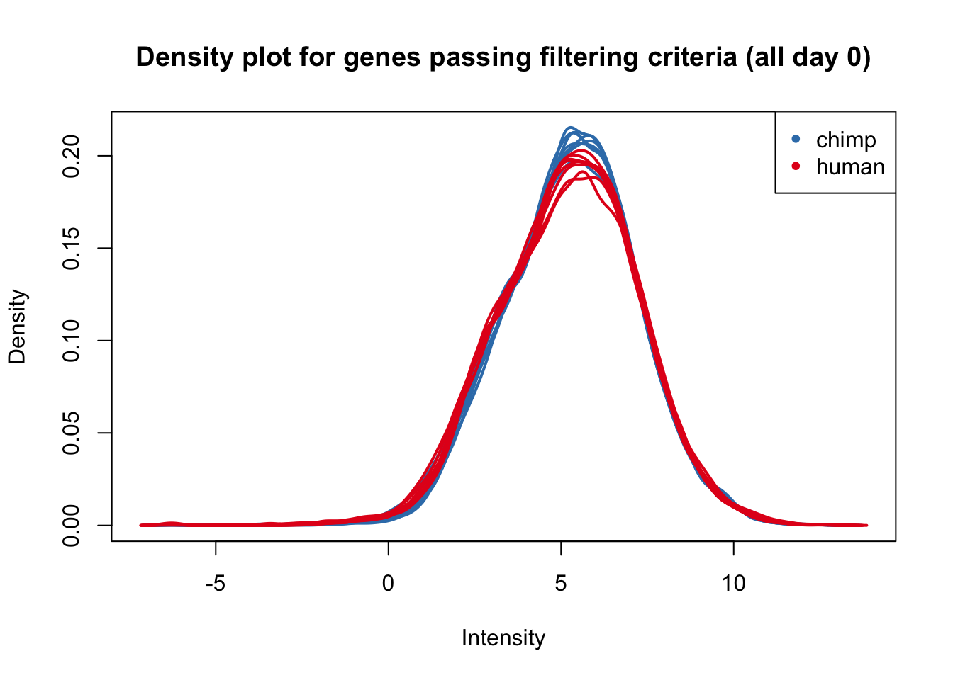
plotDensities(cpm_in_cutoff[,all_day1], col=col_day1, legend = FALSE, main = "Density plot for genes passing filtering criteria (all day 1)")
legend('topright', legend = levels(group_day1), col = levels(col_day1), pch = 20)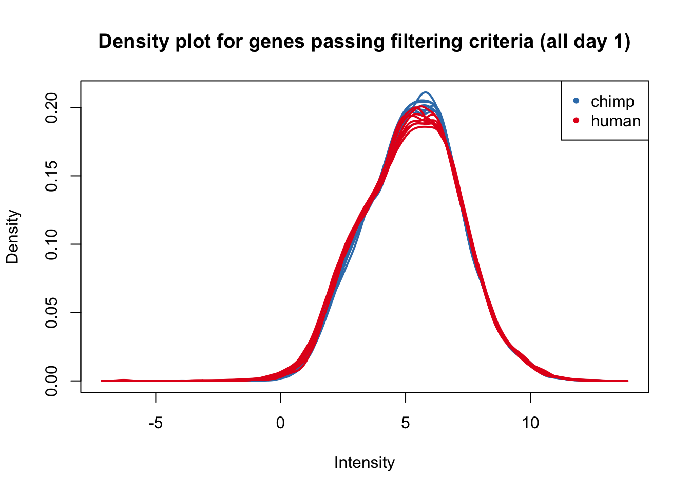
plotDensities(cpm_in_cutoff[,all_day2], col=col_day2, legend = FALSE, main = "Density plot for genes passing filtering criteria (all day 2)")
legend('topright', legend = levels(group_day2), col = levels(col_day2), pch = 20)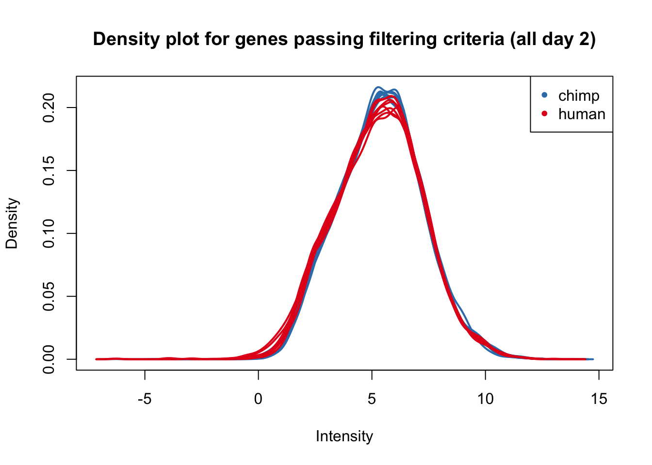
plotDensities(cpm_in_cutoff[,all_day3], col=col_day3, legend = FALSE, main = "Density plot for genes passing filtering criteria (all day 3)")
legend('topright', legend = levels(group_day3), col = levels(col_day3), pch = 20)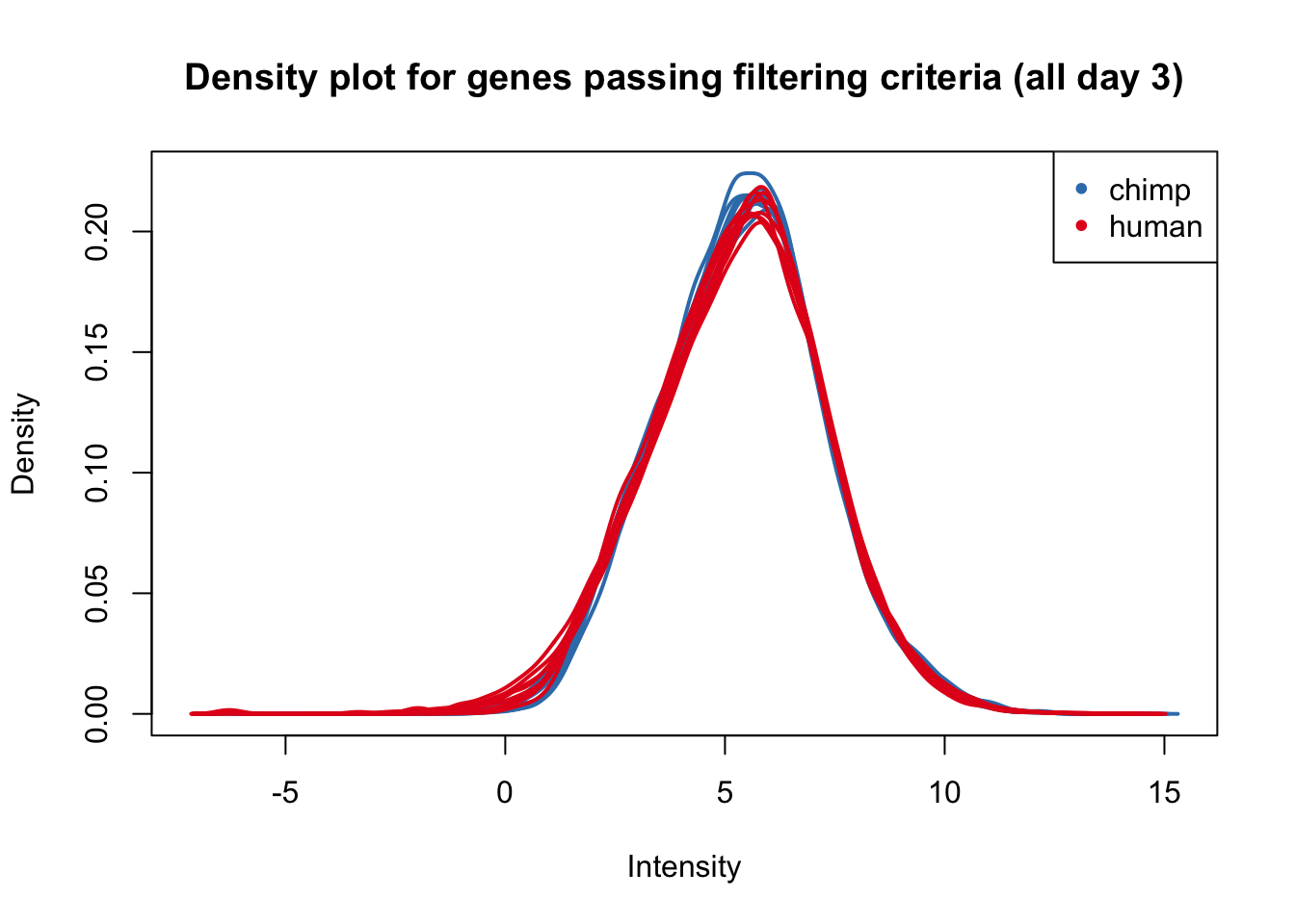
plotDensities(cpm_in_cutoff[,humans], col=col_day0, legend = FALSE, main = "Density plot for genes passing filtering criteria (all humans)")
legend('topright', legend = levels(group_humans), col = levels(col_day0), pch = 20)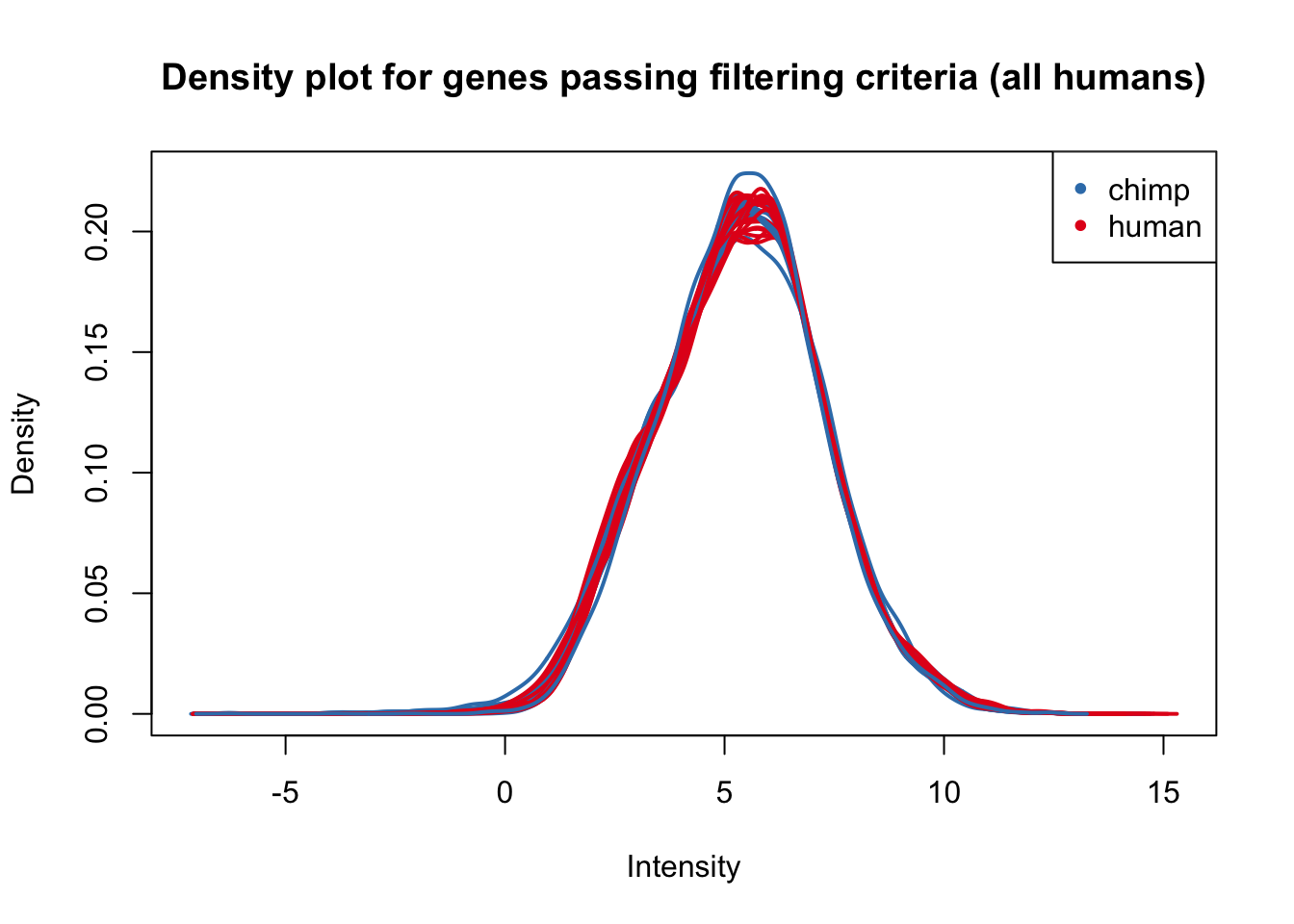
plotDensities(cpm_in_cutoff[,humans], legend = FALSE, main = "Density plot for genes passing filtering criteria (all humans)")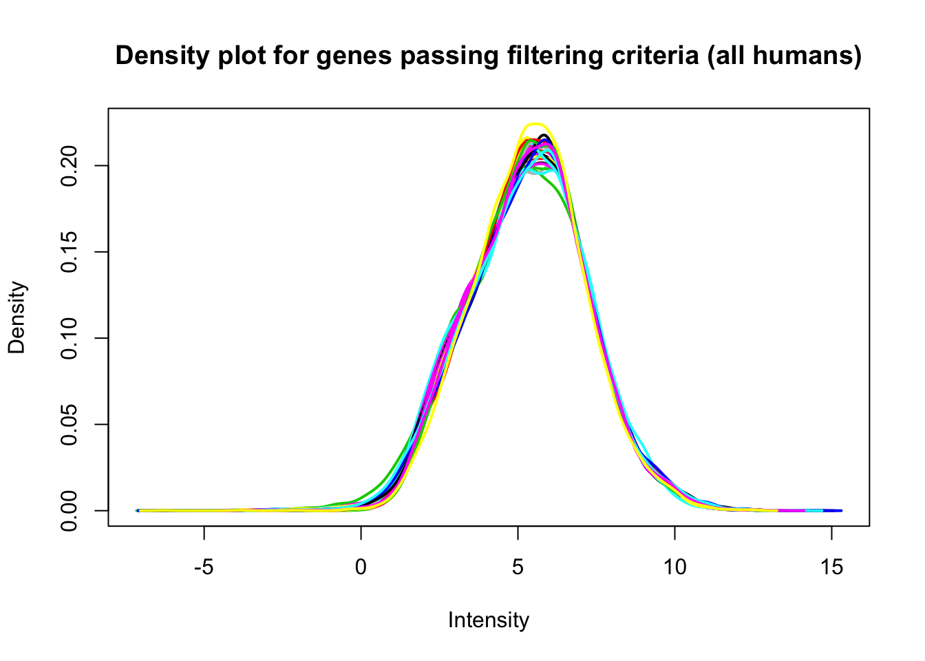
plotDensities(cpm_in_cutoff[,chimps], legend = FALSE, main = "Density plot for genes passing filtering criteria (all chimps)")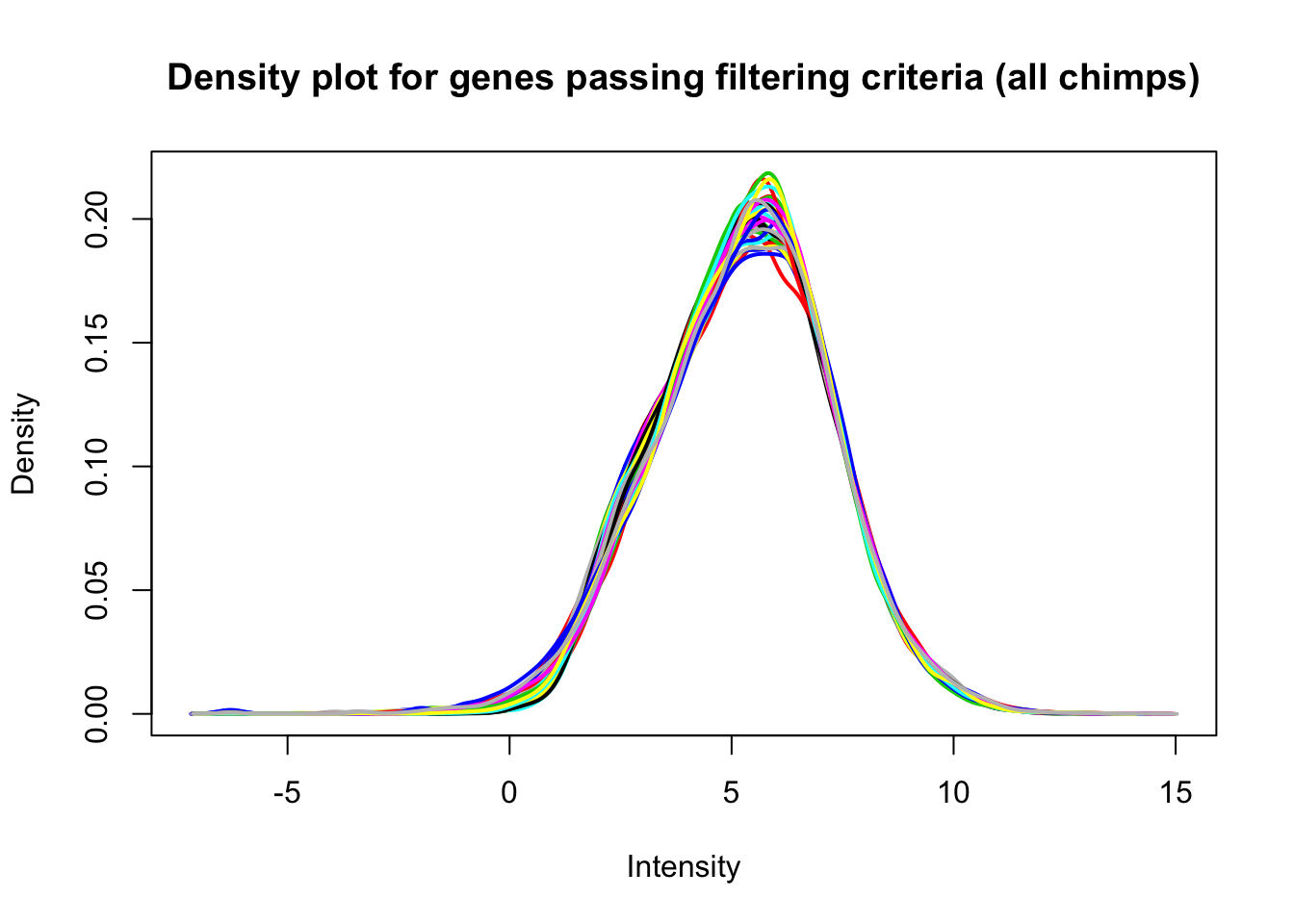
species <- c("H", "H","H","H","H","H","H", "C", "C","C","C","C","C","C","C","H","H","H","H","H","H","H","H",  "C", "C","C","C","C","C","C","C", "H","H","H","H","H","H","H","H",  "C", "C","C","C","C","C","C","C", "H","H","H","H","H","H","H","H",  "C", "C","C","C","C","C","C","C")

day <- c("0", "0","0","0","0","0","0", "0", "0", "0","0","0","0","0", "0","1","1","1","1","1","1","1","1", "1","1","1","1","1","1","1","1",  "2", "2","2","2","2","2","2","2","2", "2","2","2","2","2","2","2",  "3", "3","3","3","3","3","3","3",  "3", "3","3","3","3","3","3", "3")


design <- model.matrix(~ species*day )

colnames(design)[1] <- "Intercept"
colnames(design) <- gsub("speciesH", "Human", colnames(design))
colnames(design) <- gsub(":", ".", colnames(design))
#colnames(design) <- gsub("batch2", "batch", colnames(design))

# We want a random effect term for individual. As a result, we want to run voom twice. See https://support.bioconductor.org/p/59700/

cpm.voom <- voom(dge_in_cutoff, design, normalize.method="cyclicloess")

corfit <- duplicateCorrelation(cpm.voom, design, block=individual)

corfit.correlation =   corfit$consensus.correlation

# corfit.correlation = 0.196951
cpm.voom.corfit <- voom(dge_in_cutoff, design, plot = TRUE, normalize.method= "cyclicloess", block=individual, correlation = corfit.correlation )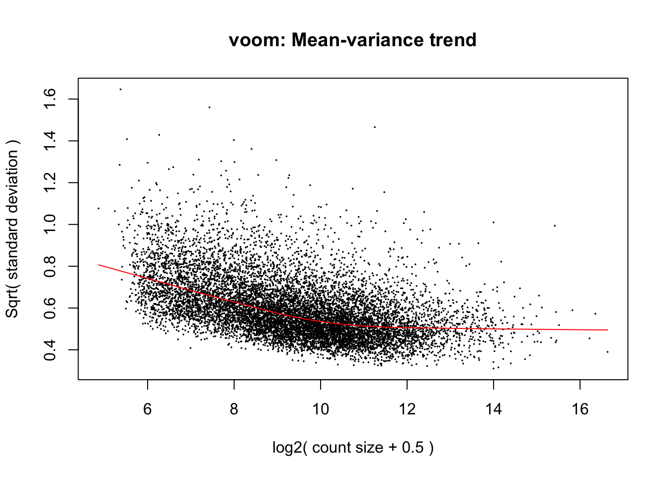
# Plot the density to see shape of the distribution

plotDensities(cpm.voom.corfit, col=pal[as.numeric(day)], legend = F)
# Run lmFit and eBayes in limma

fit <- lmFit(cpm.voom.corfit , design, block=individual, correlation=corfit.correlation)

#write.table(cpm.voom.corfit$E, file="~/Desktop/Endoderm_TC/ashlar-trial/data/cpm_cyclicloess.txt",sep="\t", col.names = T, row.names = T)


plotDensities(cpm.voom.corfit[,all_day0], col=col_day0, legend = FALSE, main = "Density plot for genes passing filtering criteria (all day 0)")
legend('topright', legend = levels(group_day0), col = levels(col_day0), pch = 20)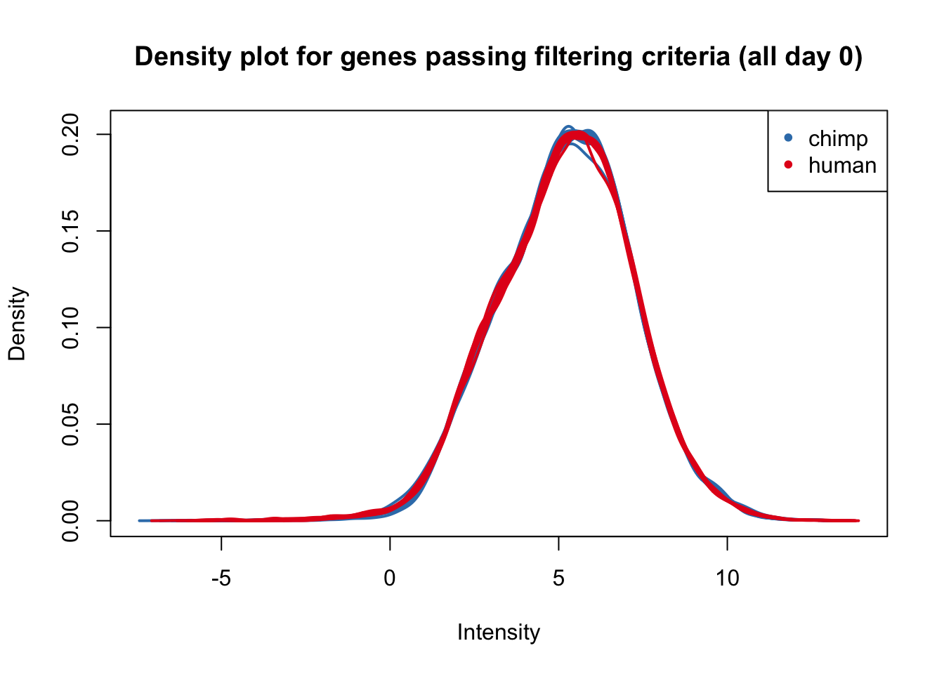
plotDensities(cpm.voom.corfit[,all_day1], col=col_day1, legend = FALSE, main = "Density plot for genes passing filtering criteria (all day 1)")
legend('topright', legend = levels(group_day1), col = levels(col_day1), pch = 20)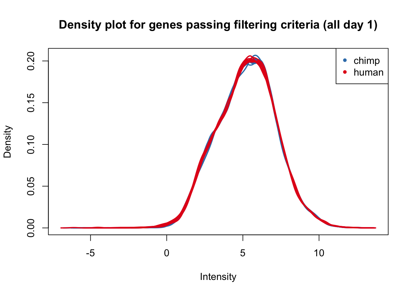
plotDensities(cpm.voom.corfit[,all_day2], col=col_day2, legend = FALSE, main = "Density plot for genes passing filtering criteria (all day 2)")
legend('topright', legend = levels(group_day2), col = levels(col_day2), pch = 20)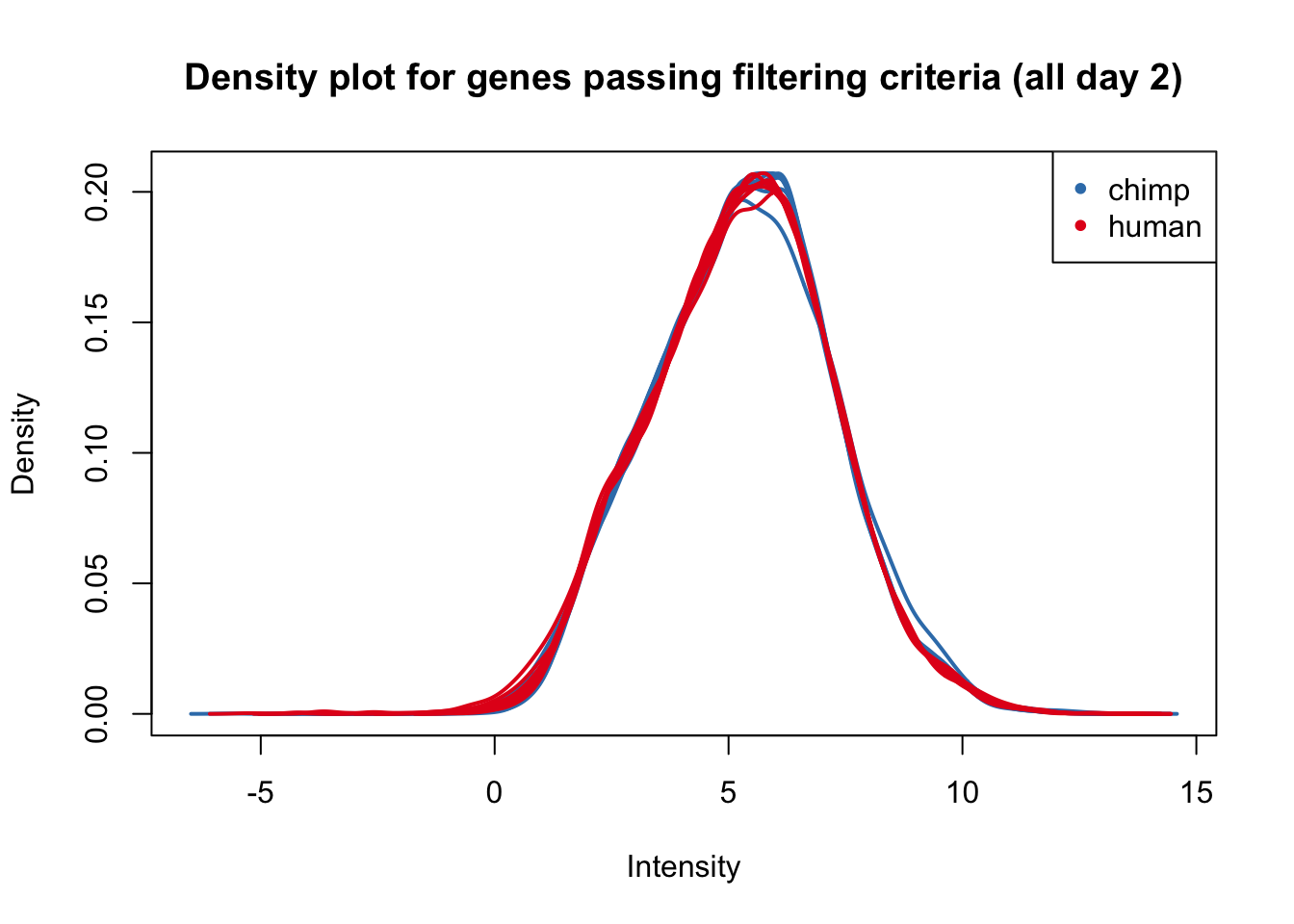
plotDensities(cpm.voom.corfit[,all_day3], col=col_day3, legend = FALSE, main = "Density plot for genes passing filtering criteria (all day 3)")
legend('topright', legend = levels(group_day3), col = levels(col_day3), pch = 20)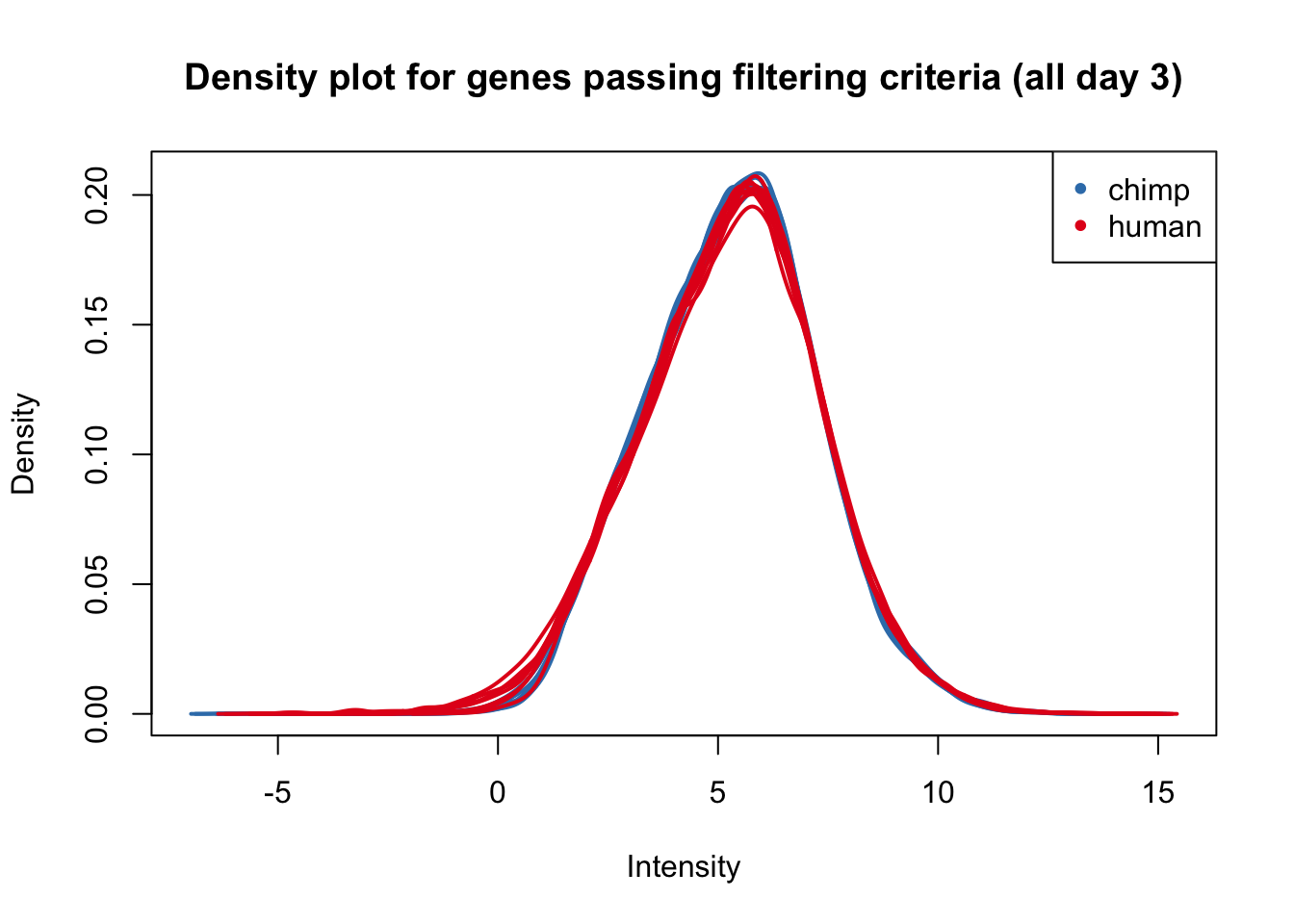
TF figures and heatmap (main paper)
### TF heatmap (main paper)

# HHEX (ENSG00000152804)

exp <- as.data.frame(cpm.voom.corfit$E[grepl("ENSG00000152804", rownames(cpm.voom.corfit$E)), ])


make_exp_df <- as.data.frame(cbind(exp, day, species))
colnames(make_exp_df) <- c("CPM", "Day", "Species")
ggplot(make_exp_df, aes(x=as.factor(Day), y=CPM, fill=Species)) + geom_boxplot(aes(fill=Species)) + ggtitle("HHEX Expression") + xlab("Day") + ylab("Normalized expression")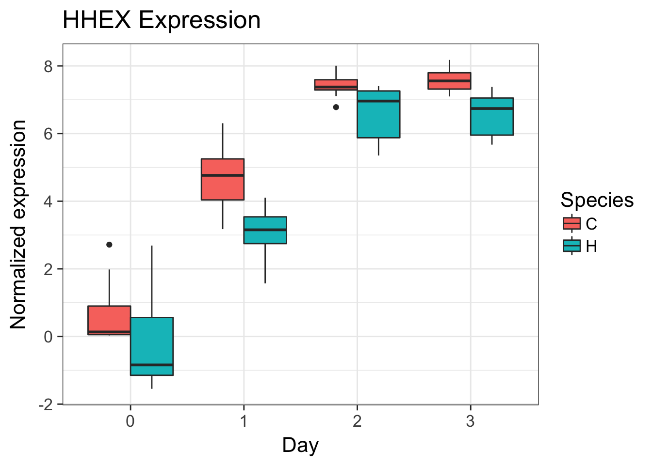
# LHX1 (ENSG00000132130)

exp <- as.data.frame(cpm.voom.corfit$E[grepl("ENSG00000132130", rownames(cpm.voom.corfit$E)), ])


make_exp_df <- as.data.frame(cbind(exp, day, species))
colnames(make_exp_df) <- c("CPM", "Day", "Species")
ggplot(make_exp_df, aes(x=as.factor(Day), y=CPM, fill=Species)) + geom_boxplot(aes(fill=Species)) + ggtitle("LHX1 Expression") + xlab("Day") + ylab("Normalized expression")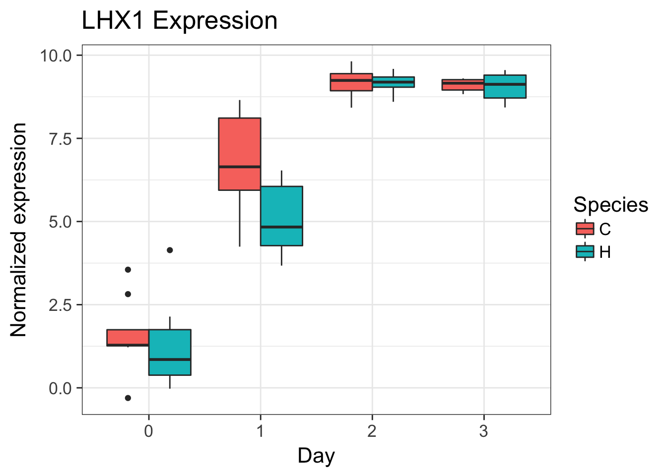
# PRDM14 (ENSG00000147596)

exp <- as.data.frame(cpm.voom.corfit$E[grepl("ENSG00000147596", rownames(cpm.voom.corfit$E)), ])


make_exp_df <- as.data.frame(cbind(exp, day, species))
colnames(make_exp_df) <- c("CPM", "Day", "Species")
ggplot(make_exp_df, aes(x=as.factor(Day), y=CPM, fill=Species)) + geom_boxplot(aes(fill=Species)) + ggtitle("PRDM14 Expression") + xlab("Day") + ylab("Normalized expression")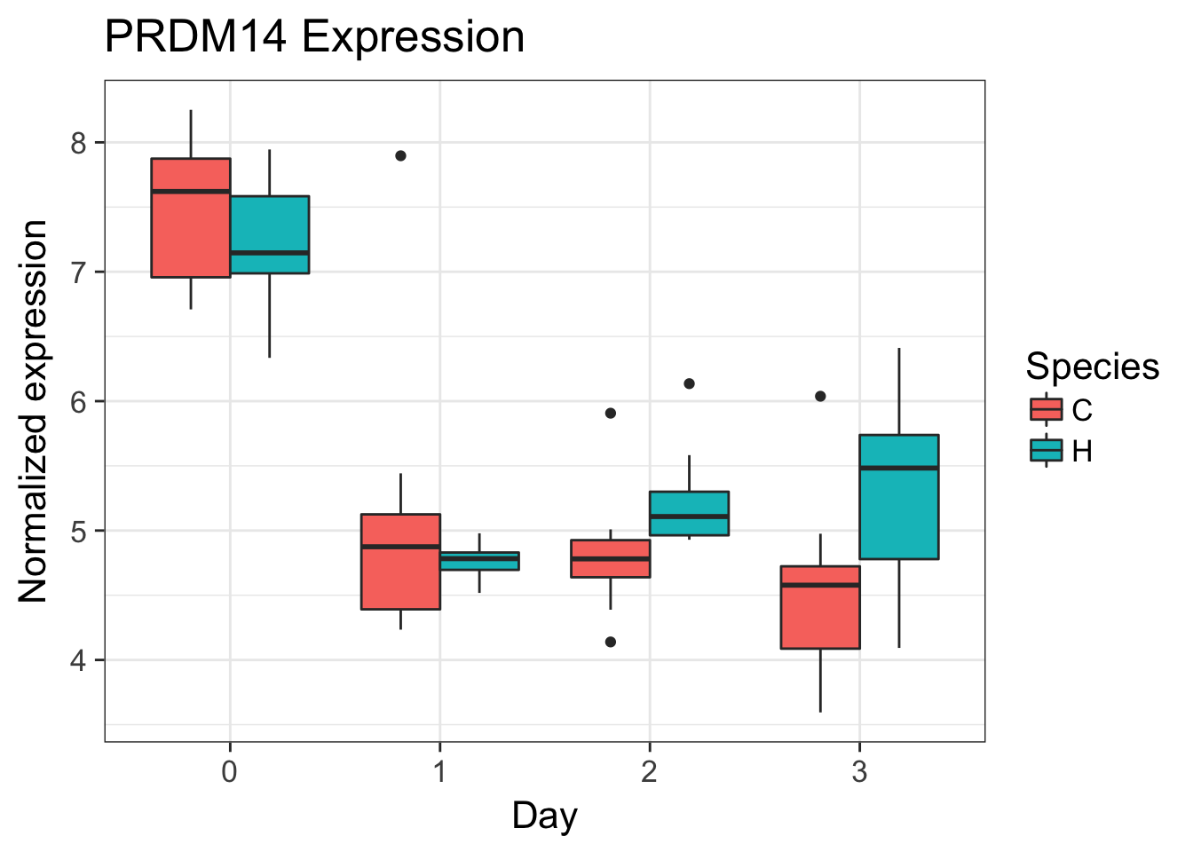
#KITLG ENSG00000049130

exp_KITLG <- as.data.frame(cpm_in_cutoff[grepl("ENSG00000049130", rownames(cpm_in_cutoff)), ])

make_exp_df <- as.data.frame(cbind(exp_KITLG, day, Species))
colnames(make_exp_df) <- c("CPM", "Day", "Species")
ggplot(make_exp_df, aes(x=as.factor(Day), y=CPM, fill=Species)) + geom_boxplot(aes(fill=as.factor(Species))) + ggtitle("KITLG Expression") + xlab("Day") +  ylab("Normalized expression") + theme_bw() + bjp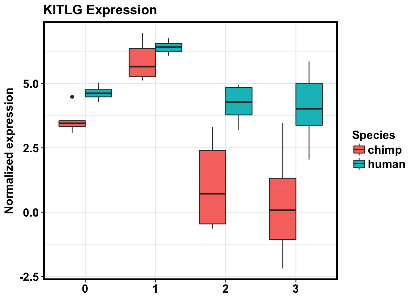
#KITLG ENSG00000049130

# ENSG00000104313
# ENSG00000137486


# ENSG00000143171
# Plot data
exp_KITLG <- as.data.frame(cpm_in_cutoff[grepl("ENSG00000104313", rownames(cpm_in_cutoff)), ])

make_exp_df <- as.data.frame(cbind(exp_KITLG, day, Species))
colnames(make_exp_df) <- c("CPM", "Day", "Species")
ggplot(make_exp_df, aes(x=as.factor(Day), y=CPM, fill=Species)) + geom_boxplot(aes(fill=as.factor(Species))) + ggtitle("EYA1 Expression") + xlab("Day") +  ylab("Normalized expression") + theme_bw() + bjp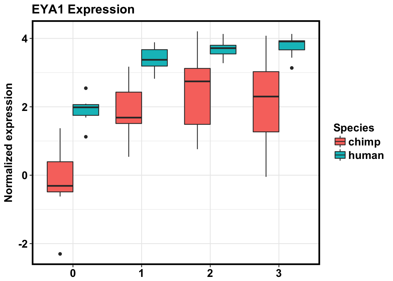
# Standardize then plot
exp_KITLG
cpm_in_cutoff[grepl("ENSG00000104313", rownames(cpm_in_cutoff)), ]
D0_20157 2.09108286
D0_20961 2.03905733
D0_21792 1.98506373
D0_28162 2.54441171
D0_28815 1.68636091
D0_28815_0116 1.81360219
D0_29089 1.12387965
D0_3647 1.37353819
D0_36470116 0.98405603
D0_3649 -0.62239112
D0_3649_0116 -2.30149725
D0_40300 -0.22462442
D0_40300_0116 0.19665694
D0_4955 -0.39779481
D0_4955_0116 -0.44261278
D1_20157 3.66108064
D1_20157_0116 3.29919607
D1_20961 3.43324856
D1_21792 3.70167896
D1_28162 2.86575463
D1_28815 3.88648205
D1_28815_0116 3.31620138
D1_29089 2.82126814
D1_3647 3.05972010
D1_3647_0116 3.17305923
D1_3649 1.27292232
D1_3649_0116 0.53827113
D1_40300 1.71371953
D1_40300_0116 1.65506626
D1_4955 1.59136843
D1_4955_0116 2.21888439
D2_20157 3.32546307
D2_20157_0116 3.72517542
D2_20961 3.78472350
D2_21792 4.12985672
D2_28162 3.62039124
D2_28815 3.84381130
D2_28815_0116 3.70507413
D2_29089 3.27632944
D2_3647 4.20660412
D2_3647_0116 2.78034276
D2_3649 0.76107868
D2_3649_0116 0.86581427
D2_40300 2.99459978
D2_40300_0116 3.50647908
D2_4955 1.69326807
D2_4955_0116 2.70662259
D3_20157 3.91236664
D3_20157_0116 3.91678760
D3_20961 3.74157476
D3_21792 3.43674479
D3_28162 3.90839067
D3_28815 4.13044226
D3_28815_0116 3.97433118
D3_29089 3.13621798
D3_3647 4.07820463
D3_3647_0116 2.44792638
D3_3649 0.17644205
D3_3649_0116 -0.04834571
D3_40300 2.15289077
D3_40300_0116 3.45945683
D3_4955 1.63054490
D3_4955_0116 2.88421146humans <- c(1:7, 16:23, 32:39, 48:55)
chimps <- c(8:15, 24:31, 40:47, 56:63)
mean_day0_humans <- mean(exp_KITLG[1:7,] )
mean_day0_chimps <- mean(exp_KITLG[8:15,] )
day0humans <- as.data.frame(exp_KITLG[1:7,] - 0.897)
colnames(day0humans) <- c("standardized mean")
day0chimps <- as.data.frame(exp_KITLG[8:15,] + 1.179)
colnames(day0chimps) <- c("standardized mean")
day1humans <- as.data.frame(exp_KITLG[16:23,] - 0.897)
colnames(day1humans) <- c("standardized mean")
day1chimps <- as.data.frame(exp_KITLG[24:31,] + 1.179)
colnames(day1chimps) <- c("standardized mean")
day2humans <- as.data.frame(exp_KITLG[32:39,] - 0.897)
colnames(day2humans) <- c("standardized mean")
day2chimps <- as.data.frame(exp_KITLG[40:47,] + 1.179)
colnames(day2chimps) <- c("standardized mean")
day3humans <- as.data.frame(exp_KITLG[48:55,] - 0.897)
colnames(day3humans) <- c("standardized mean")
day3chimps <- as.data.frame(exp_KITLG[56:63,] + 1.79)
colnames(day3chimps) <- c("standardized mean")
exp_stand <- rbind(day0humans, day0chimps, day1humans, day1chimps, day2humans, day2chimps, day3humans, day3chimps)
make_exp_df <- as.data.frame(cbind(exp_stand, day, Species))
colnames(make_exp_df) <- c("CPM", "Day", "Species")
ggplot(make_exp_df, aes(x=as.factor(Day), y=CPM, fill=Species)) + geom_boxplot(aes(fill=as.factor(Species))) + ggtitle("Standardized EYA1 Expression") + xlab("Day") + ylab("Standardized expression") + theme_bw() + bjp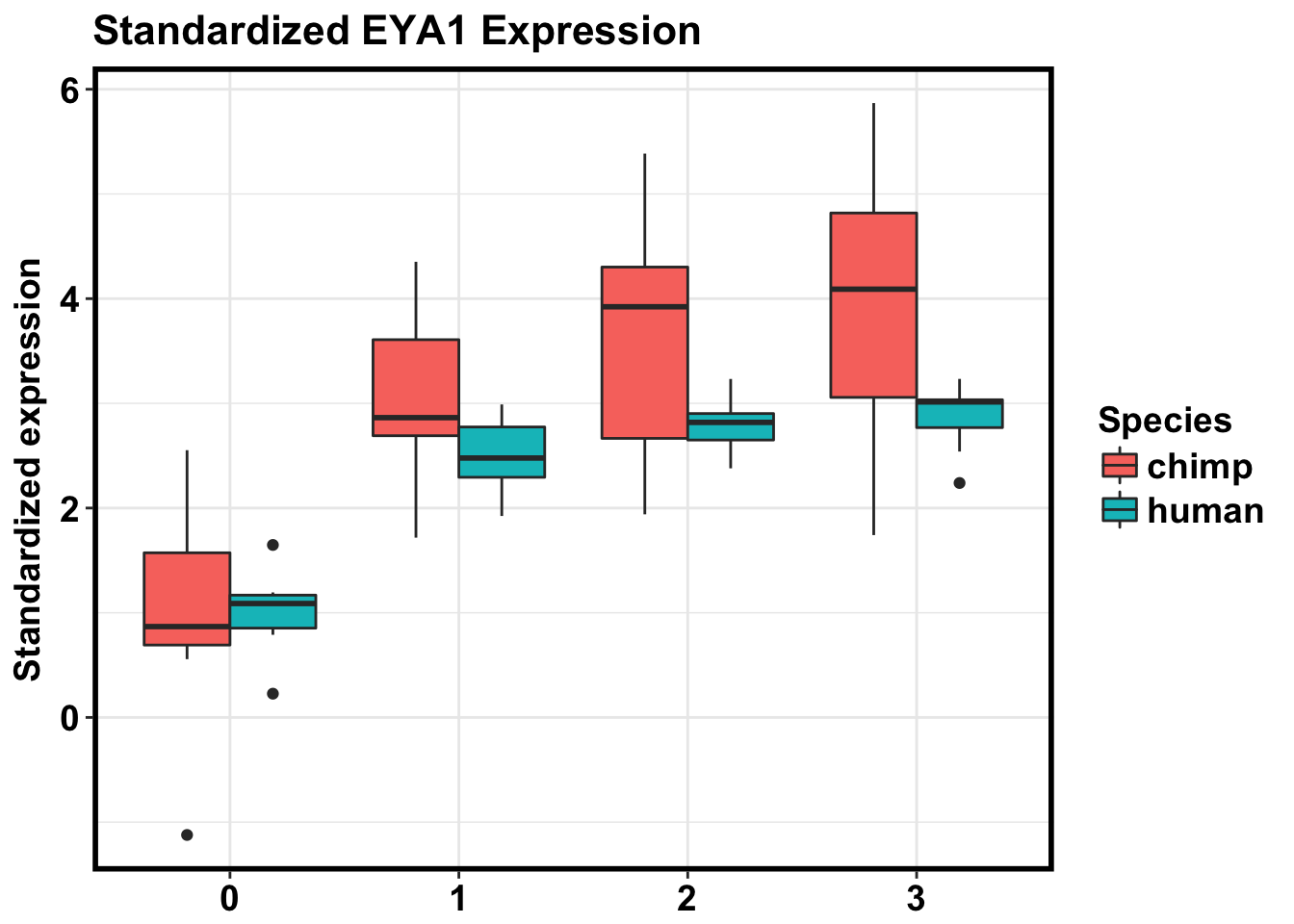
# Note: ELAC2 is gene 105

gene_105 <- as.data.frame(cpm_in_cutoff[105, ] )

make_exp_df <- as.data.frame(cbind(gene_105, day, Species))
colnames(make_exp_df) <- c("CPM", "Day", "Species")
ggplot(make_exp_df, aes(x=as.factor(Day), y=CPM, fill=Species)) + geom_boxplot(aes(fill=as.factor(Species))) + ggtitle("ELAC2 Expression") + xlab("Day") +  ylab("Normalized expression") + theme_bw() + bjp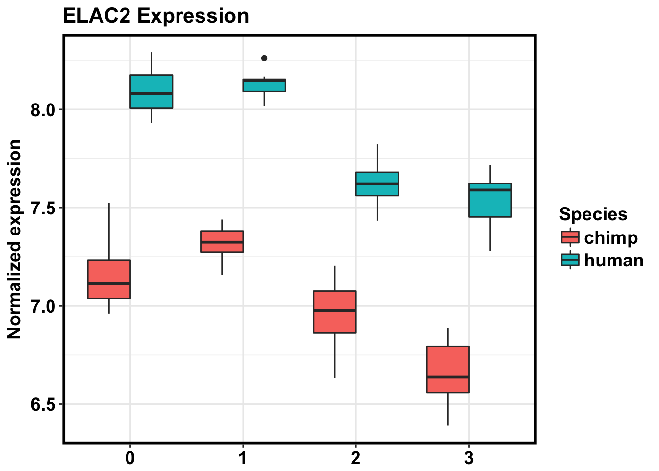
# Standardization - 110, 111, 116, 121, 125, 139
gene_105 <- as.data.frame(cpm_in_cutoff[151, ] )

make_exp_df <- as.data.frame(cbind(gene_105, day, Species))
colnames(make_exp_df) <- c("CPM", "Day", "Species")
ggplot(make_exp_df, aes(x=as.factor(Day), y=CPM, fill=Species)) + geom_boxplot(aes(fill=as.factor(Species)), show.legend = FALSE) + ggtitle("RPS20 Gene Expression") + xlab("Day") +  ylab("Normalized expression") + theme_bw() + bjp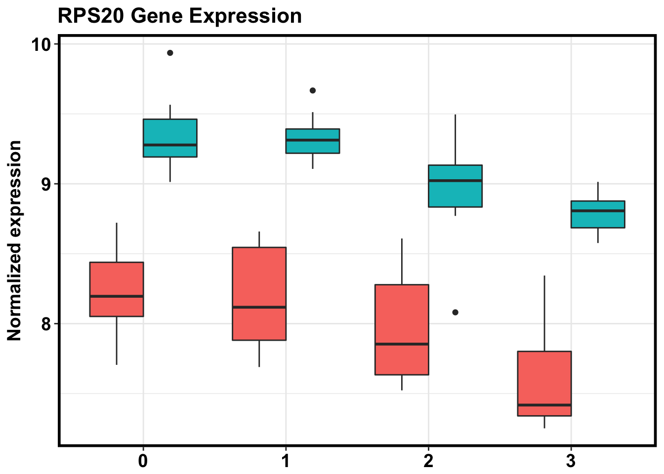
mean_day0_humans <- median(gene_105[1:7,] )
mean_day0_chimps <- median(gene_105[8:15,] )

day0humans <- as.data.frame(gene_105[1:7,] - mean_day0_humans + 1)
colnames(day0humans) <- c("standardized mean")
day0chimps <- as.data.frame(gene_105[8:15,] - mean_day0_chimps + 1)
colnames(day0chimps) <- c("standardized mean")
day1humans <- as.data.frame(gene_105[16:23,] - mean_day0_humans + 1)
colnames(day1humans) <- c("standardized mean")
day1chimps <- as.data.frame(gene_105[24:31,]  - mean_day0_chimps + 1)
colnames(day1chimps) <- c("standardized mean")
day2humans <- as.data.frame(gene_105[32:39,] - mean_day0_humans + 1)
colnames(day2humans) <- c("standardized mean")
day2chimps <- as.data.frame(gene_105[40:47,] - mean_day0_chimps + 1)
colnames(day2chimps) <- c("standardized mean")
day3humans <- as.data.frame(gene_105[48:55,] - mean_day0_humans + 1)
colnames(day3humans) <- c("standardized mean")
day3chimps <- as.data.frame(gene_105[56:63,] - mean_day0_chimps + 1)
colnames(day3chimps) <- c("standardized mean")

exp_stand <- rbind(day0humans, day0chimps, day1humans, day1chimps, day2humans, day2chimps, day3humans, day3chimps)

make_exp_df <- as.data.frame(cbind(exp_stand, day, Species))
colnames(make_exp_df) <- c("CPM", "Day", "Species")
ggplot(make_exp_df, aes(x=as.factor(Day), y=CPM, fill=Species)) + geom_boxplot(aes(fill=as.factor(Species)), show.legend = FALSE) + ggtitle("Standardized RPS20 Gene Expression") + xlab("Day") +  ylab("Standardized expression") + theme_bw() + bjp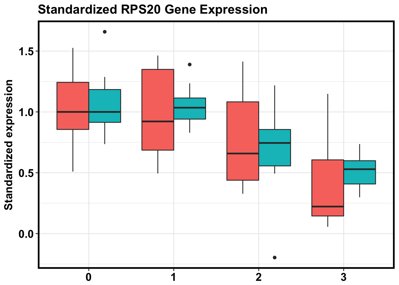
# reduction in variance
red_var <- as.data.frame(cpm_in_cutoff[2, ] )

make_exp_df <- as.data.frame(cbind(red_var, day, Species))
colnames(make_exp_df) <- c("CPM", "Day", "Species")
ggplot(make_exp_df, aes(x=as.factor(Day), y=CPM, fill=Species)) + geom_boxplot(aes(fill=as.factor(Species))) + ggtitle("KITLG Expression") + xlab("Day") +  ylab("Normalized expression") + theme_bw() + bjp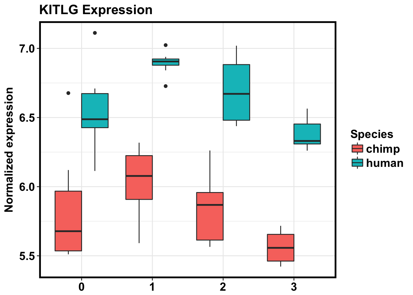
cpm_in_cutoff <- cpm.voom.corfit$E

# New heatmap

# EOMES (ENSG00000163508)

exp_EOMES <- as.data.frame(cpm_in_cutoff[grepl("ENSG00000163508", rownames(cpm_in_cutoff)), ])

make_exp_df <- as.data.frame(cbind(t(exp_EOMES), day, Species))
Warning in cbind(t(exp_EOMES), day, Species): number of rows of result is
not a multiple of vector length (arg 2)colnames(make_exp_df) <- c("CPM", "Day", "Species")
ggplot(make_exp_df, aes(x=as.factor(Day), y=CPM, fill=Species)) + geom_boxplot(aes(fill=as.factor(Species))) + ggtitle("EOMES Expression") + xlab("Day") + ylab("Normalized expression") + theme_bw() + bjp
# GSC (ENSG00000133937)

exp_GSC <- as.data.frame(cpm_in_cutoff[grepl("ENSG00000133937", rownames(cpm_in_cutoff)), ])


# EOMES (ENSG00000141448)

exp_GATA6 <- as.data.frame(cpm_in_cutoff[grepl("ENSG00000141448", rownames(cpm_in_cutoff)), ])

# FOXA2 (ENSG00000125798)

exp_FOXA2 <- as.data.frame(cpm_in_cutoff[grepl("ENSG00000125798", rownames(cpm_in_cutoff)), ])

# CER1 (ENSG00000147869)

exp_CER1 <- as.data.frame(cpm_in_cutoff[grepl("ENSG00000147869", rownames(cpm_in_cutoff)), ])

# Nodal (ENSG00000156574)

exp_NODAL <- as.data.frame(cpm_in_cutoff[grepl("ENSG00000156574", rownames(cpm_in_cutoff)), ])

# WNT3 (ENSG00000108379)

exp_WNT3 <- as.data.frame(cpm_in_cutoff[grepl("ENSG00000108379", rownames(cpm_in_cutoff)), ])

# MIXL1 (ENSG00000185155)

exp_MIXL1 <- as.data.frame(cpm_in_cutoff[grepl("ENSG00000185155", rownames(cpm_in_cutoff)), ])

# SNAI1 (ENSG00000124216)

exp_SNAI1 <- as.data.frame(cpm_in_cutoff[grepl("ENSG00000124216", rownames(cpm_in_cutoff)), ])

# HHEX (ENSG00000152804)

exp_HHEX <- as.data.frame(cpm_in_cutoff[grepl("ENSG00000152804", rownames(cpm_in_cutoff)), ])

# CXCR4 (ENSG00000121966)

exp_CXCR4 <- as.data.frame(cpm_in_cutoff[grepl("ENSG00000121966", rownames(cpm_in_cutoff)), ])

# SOX17 (ENSG00000164736)

exp_SOX17 <- as.data.frame(cpm_in_cutoff[grepl("ENSG00000164736", rownames(cpm_in_cutoff)), ])

# KLF8 (ENSG00000102349)

exp_KLF8 <- as.data.frame(cpm_in_cutoff[grepl("ENSG00000102349", rownames(cpm_in_cutoff)), ])

# OTX2 (ENSG00000165588)

exp_OTX2 <- as.data.frame(cpm_in_cutoff[grepl("ENSG00000165588", rownames(cpm_in_cutoff)), ])

# PRDM1 (ENSG00000057657)

exp_PRDM1 <- as.data.frame(cpm_in_cutoff[grepl("ENSG00000057657", rownames(cpm_in_cutoff)), ])

# KIT (ENSG00000157404)

exp_KIT <- as.data.frame(cpm_in_cutoff[grepl("ENSG00000157404", rownames(cpm_in_cutoff)), ])

# FOXM1 (ENSG00000111206)

exp_FOXM1 <- as.data.frame(cpm_in_cutoff[grepl("ENSG00000111206", rownames(cpm_in_cutoff)), ])

# BRACHYURY (ENSG00000164458)

exp_BRACHYURY <- as.data.frame(cpm_in_cutoff[grepl("ENSG00000164458", rownames(cpm_in_cutoff)), ])

# SHISA2 (ENSG00000180730)

exp_SHISA2 <- as.data.frame(cpm_in_cutoff[grepl("ENSG00000180730", rownames(cpm_in_cutoff)), ])

# CDH1 (ENSG00000039068)

exp_CDH1 <- as.data.frame(cpm_in_cutoff[grepl("ENSG00000039068", rownames(cpm_in_cutoff)), ])

# CDH2 (ENSG00000170558)

exp_CDH2 <- as.data.frame(cpm_in_cutoff[grepl("ENSG00000170558", rownames(cpm_in_cutoff)), ])

# PRDM14 (ENSG00000147596)

exp_PRDM14 <- as.data.frame(cpm_in_cutoff[grepl("ENSG00000147596", rownames(cpm_in_cutoff)), ])

# WNT5A (ENSG00000114251)

exp_WNT5A <- as.data.frame(cpm_in_cutoff[grepl("ENSG00000114251", rownames(cpm_in_cutoff)), ])

# WNT5B (ENSG00000111186)

exp_WNT5B <- as.data.frame(cpm_in_cutoff[grepl("ENSG00000111186", rownames(cpm_in_cutoff)), ])

# SOX2 (ENSG00000181449)

exp_SOX2 <- as.data.frame(cpm_in_cutoff[grepl("ENSG00000181449", rownames(cpm_in_cutoff)), ])

# PDGFRA (ENSG00000134853)

exp_PDGFRA <- as.data.frame(cpm_in_cutoff[grepl("ENSG00000134853", rownames(cpm_in_cutoff)), ])

# DKK1 (ENSG00000107984)

exp_DKK1 <- as.data.frame(cpm_in_cutoff[grepl("ENSG00000107984", rownames(cpm_in_cutoff)), ])

# DKK4 (ENSG00000104371)

exp_DKK4 <- as.data.frame(cpm_in_cutoff[grepl("ENSG00000104371", rownames(cpm_in_cutoff)), ])

# FGF8 (ENSG00000107831)

exp_FGF8 <- as.data.frame(cpm_in_cutoff[grepl("ENSG00000107831", rownames(cpm_in_cutoff)), ])


TF_heatmap <- cbind(exp_EOMES, exp_GSC, exp_GATA6, exp_FOXA2, exp_CER1, exp_NODAL, exp_WNT3, exp_MIXL1, exp_SNAI1, exp_HHEX, exp_CXCR4, exp_SOX17, exp_KLF8, exp_OTX2, exp_PRDM1, exp_KIT, exp_FOXM1, exp_BRACHYURY, exp_SHISA2, exp_CDH1, exp_CDH2, exp_PRDM14, exp_WNT5A, exp_WNT5B, exp_SOX2, exp_PDGFRA, exp_DKK1, exp_DKK4,  exp_FGF8)
colnames(TF_heatmap) <- c("EOMES", "GSC", "GATA6", "FOXA2", "CER1", "NODAL", "WNT3", "MIXL1", "SNAI1", "HHEX", "CXCR4", "SOX17", "KLF8", "OTX2", "PRDM1", "KIT", "FOXM1", "BRACHYURY", "SHISA2", "CDH1", "CDH2", "PRDM14", "WNT5A", "WNT5B", "SOX2", "PDGFRA", "DKK1", "DKK4",  "FGF8")

dim(TF_heatmap)
[1] 63 29gplots::heatmap.2(x=as.matrix(t(TF_heatmap)),
# , distfun = dist(x, method = "euclidean"),
hclustfun = function(x) hclust(dist(x), method = "average"), tracecol=NA, col=colors, denscol="white", labCol= labels, ColSideColors=pal[as.integer(as.factor(day))])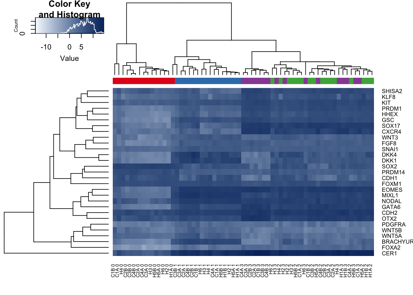
Data visualization
# Make PCA plots with the factors colored by day

cpm_cyclicloess <- read.table("~/Desktop/Endoderm_TC/ashlar-trial/data/cpm_cyclicloess.txt")

pca_genes <- prcomp(t(cpm_cyclicloess), scale = T, retx = TRUE, center = TRUE)
scores <- pca_genes$x

matrixpca <- pca_genes$x
pc1 <- matrixpca[,1]
pc2 <- matrixpca[,2]
pc3 <- matrixpca[,3]
pc4 <- matrixpca[,4]
pc5 <- matrixpca[,5]

pcs <- data.frame(pc1, pc2, pc3, pc4, pc5)

summary <- summary(pca_genes)

# Correlations
cor(pc1, as.numeric(day))
[1] 0.9245192cor(pc2, as.numeric(as.factor(species)))[1] 0.9329493ggplot(data=pcs, aes(x=pc1, y=pc2, color=as.factor(day), shape=as.factor(species), size=2)) + geom_point() + xlab(paste("PC1 (",(summary$importance[2,1]*100), "% of variance)")) + ylab(paste("PC2 (",(summary$importance[2,2]*100), "% of variance)")) + guides(color = guide_legend(order=1), size = FALSE, shape = guide_legend(order=2)) + scale_color_discrete(name ="Day") + labs(title = "PCA of normalized endoderm data ")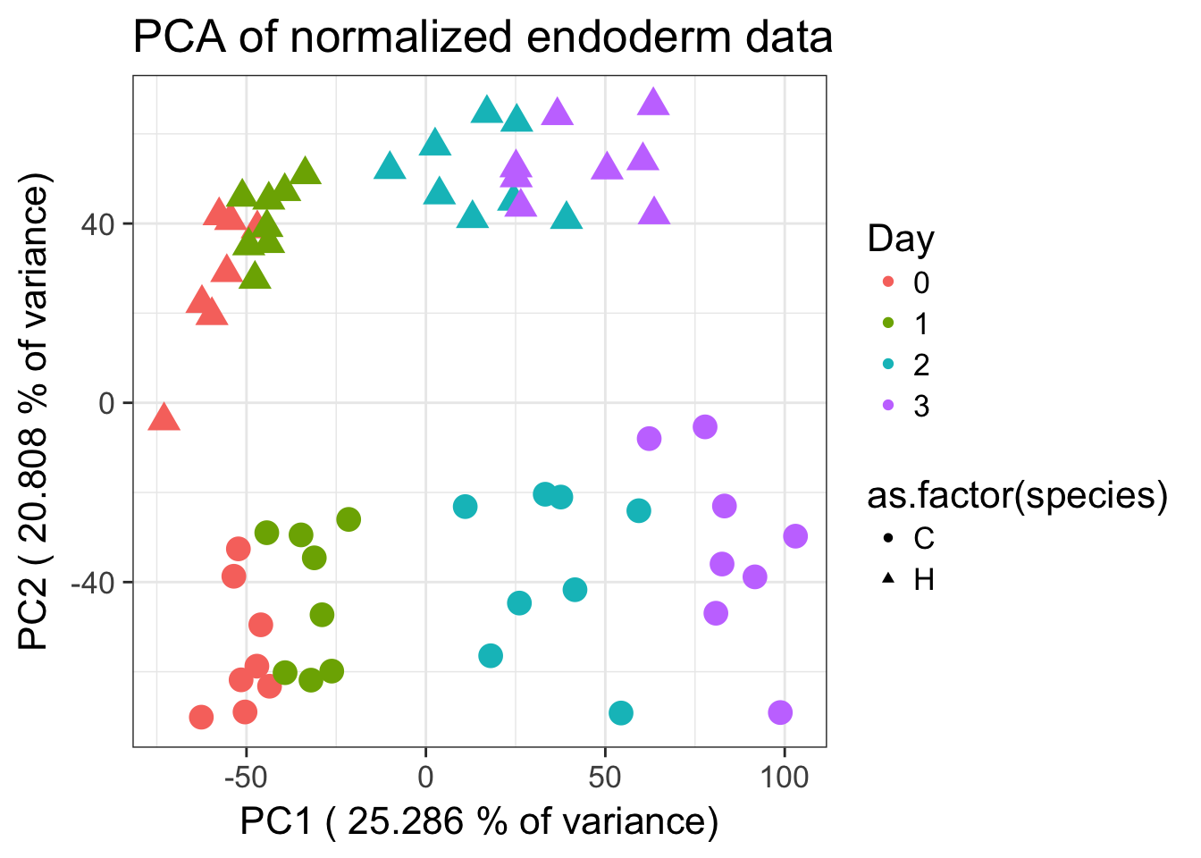
Final, no global (5% FDR, main paper)
species <- c("H", "H","H","H","H","H","H", "C", "C","C","C","C","C","C","C","H","H","H","H","H","H","H","H",  "C", "C","C","C","C","C","C","C", "H","H","H","H","H","H","H","H",  "C", "C","C","C","C","C","C","C", "H","H","H","H","H","H","H","H",  "C", "C","C","C","C","C","C","C")

day <- c("0", "0","0","0","0","0","0", "0", "0", "0","0","0","0","0", "0","1","1","1","1","1","1","1","1", "1","1","1","1","1","1","1","1",  "2", "2","2","2","2","2","2","2","2", "2","2","2","2","2","2","2",  "3", "3","3","3","3","3","3","3",  "3", "3","3","3","3","3","3", "3")


design <- model.matrix(~ species*day )

colnames(design)[1] <- "Intercept"
colnames(design) <- gsub("speciesH", "Human", colnames(design))
colnames(design) <- gsub(":", ".", colnames(design))
#colnames(design) <- gsub("batch2", "batch", colnames(design))

# We want a random effect term for individual. As a result, we want to run voom twice. See https://support.bioconductor.org/p/59700/

cpm.voom <- voom(dge_in_cutoff, design, normalize.method="cyclicloess")

corfit <- duplicateCorrelation(cpm.voom, design, block=individual)

corfit.correlation =   corfit$consensus.correlation

cpm.voom.corfit <- voom(dge_in_cutoff, design, plot = TRUE, normalize.method="cyclicloess", block=individual, correlation = corfit.correlation )
# Plot the density to see shape of the distribution

plotDensities(cpm.voom.corfit, col=pal[as.numeric(day)], legend = F)
# Run lmFit and eBayes in limma

fit <- lmFit(cpm.voom.corfit , design, block=individual, correlation=corfit.correlation)


# In the contrast matrix, we have the species DE at each day

cm2 <- makeContrasts(HvCday0 = Human, HvCday1 = Human + Human.day1, HvCday2 = Human + Human.day2, HvCday3 = Human + Human.day3, Hday01 = day1 + Human.day1, Hday12 = day2 + Human.day2 - day1 - Human.day1, Hday23 = day3 + Human.day3 - day2 - Human.day2, Cday01 = day1, Cday12 = day2 - day1, Cday23 = day3 - day2, Sig_inter_day1 = Human.day1, Sig_inter_day2 = Human.day2 - Human.day1, Sig_inter_day3 = Human.day3 - Human.day2, levels = design)

# Fit the new model
diff_species <- contrasts.fit(fit, cm2)
fit2 <- eBayes(diff_species)


top3 <- list(HvCday0 =topTable(fit2, coef=1, adjust="BH", number=Inf, sort.by="none"), HvCday1 =topTable(fit2, coef=2, adjust="BH", number=Inf, sort.by="none"),  HvCday2 =topTable(fit2, coef=3, adjust="BH", number=Inf, sort.by="none"),  HvCday3 =topTable(fit2, coef=4, adjust="BH", number=Inf, sort.by="none"), Hday01 =topTable(fit2, coef=5, adjust="BH", number=Inf, sort.by="none"), Hday12 =topTable(fit2, coef=6, adjust="BH", number=Inf, sort.by="none"),  Hday23 =topTable(fit2, coef=7, adjust="BH", number=Inf, sort.by="none"),  Cday01 =topTable(fit2, coef=8, adjust="BH", number=Inf, sort.by="none"), Cday12 =topTable(fit2, coef=9, adjust="BH", number=Inf, sort.by="none"), Cday23 =topTable(fit2, coef=10, adjust="BH", number=Inf, sort.by="none"), Sig_inter_day1 =topTable(fit2, coef=11, adjust="BH", number=Inf, sort.by="none"), Sig_inter_day2 =topTable(fit2, coef=12, adjust="BH", number=Inf, sort.by="none"), Sig_inter_day3 =topTable(fit2, coef=13, adjust="BH", number=Inf, sort.by="none"))

#write.table(fit2, "~/Dropbox/Endoderm TC/Cyclic_loess_norm/unscaled_SD.txt", sep="\t")


# Set FDR level at 5%

FDR_level <- 0.05
#FDR_level <- 0.01


important_columns <- c(1,2,6)

# Find the genes that are DE at Day 0
HvCday0 =topTable(fit2, coef=1, adjust="BH", number=Inf, sort.by="none")
dim(HvCday0[which(HvCday0$adj.P.Val < 0.05), important_columns])
[1] 4475 3HvCday0_adj_pval <- HvCday0[which(HvCday0$adj.P.Val < 0.05), ]
HvCday0_adj_pval <- HvCday0[, important_columns]
# Find the genes that are DE at Day 1
HvCday1 =topTable(fit2, coef=2, adjust="BH", number=Inf, sort.by="none")
dim(HvCday1[which(HvCday1$adj.P.Val < 0.05), important_columns])[1] 4408 3HvCday1_adj_pval <- HvCday1[which(HvCday1$adj.P.Val < 0.05), ]
HvCday1_adj_pval <- HvCday1[, important_columns]
# Find the genes that are DE at Day 2
HvCday2 =topTable(fit2, coef=3, adjust="BH", number=Inf, sort.by="none")
dim(HvCday2[which(HvCday2$adj.P.Val < 0.05), important_columns]) [1] 4712 3HvCday2_adj_pval <- HvCday2[which(HvCday2$adj.P.Val < 0.05), ]
HvCday2_adj_pval <- HvCday2[, important_columns]
# Find the genes that are DE at Day 3
HvCday3 =topTable(fit2, coef=4, adjust="BH", number=Inf, sort.by="none")
dim(HvCday3[which(HvCday3$adj.P.Val < 0.05), important_columns]) [1] 5077 3HvCday3_adj_pval <- HvCday3[which(HvCday3$adj.P.Val < 0.05), ]
HvCday3_adj_pval <- HvCday3[, important_columns]
#4475
#4408
#4712
#5077
dim(HvCday0_adj_pval)[1] 10304 3dim(HvCday1_adj_pval)[1] 10304 3dim(HvCday2_adj_pval)[1] 10304 3dim(HvCday3_adj_pval)[1] 10304 3#write.table(HvCday0, "~/Desktop/Endoderm_TC/ashlar-trial/data/HvC_day0_all_genes.txt", sep="\t")
#write.table(HvCday1, "~/Desktop/Endoderm_TC/ashlar-trial/data/HvC_day1_all_genes.txt", sep="\t")
#write.table(HvCday2, "~/Desktop/Endoderm_TC/ashlar-trial/data/HvC_day2_all_genes.txt", sep="\t")
#write.table(HvCday3, "~/Desktop/Endoderm_TC/ashlar-trial/data/HvC_day3_all_genes.txt", sep="\t")
# Table 2
#write.table(HvCday0_adj_pval, "~/Dropbox/Endoderm TC/Cyclic_loess_norm/Main_paper_April_18/HvC_day0_all_genes.txt", #sep="\t")
#write.table(HvCday1_adj_pval, "~/Dropbox/Endoderm TC/Cyclic_loess_norm/HvC_day1_all_genes.txt", sep="\t")
#write.table(HvCday2_adj_pval, "~/Dropbox/Endoderm TC/Cyclic_loess_norm/HvC_day2_all_genes.txt", sep="\t")
#write.table(HvCday3_adj_pval, "~/Dropbox/Endoderm TC/Cyclic_loess_norm/HvC_day3_all_genes.txt", sep="\t")
important_columns <- c(1,2,6)
# Find the genes that are DE at Human Day 0 to Day 1
H_day01 =topTable(fit2, coef=5, adjust="BH", number=Inf, sort.by="none")
dim(H_day01[which(H_day01$adj.P.Val < 0.05), important_columns])[1] 3231 3H_day01 <- H_day01[which(H_day01$adj.P.Val < 0.05), ]
# H_day01 <- H_day01[, important_columns]
# Find the genes that are DE at Human Day 1 to Day 2
H_day12 =topTable(fit2, coef=6, adjust="BH", number=Inf, sort.by="none")
dim(H_day12[which(H_day12$adj.P.Val < 0.05), important_columns])[1] 4293 3H_day12 <- H_day12[which(H_day12$adj.P.Val < 0.05), ]
# H_day12 <- H_day12[, important_columns]
# Find the genes that are DE at Human Day 2 to Day 3
H_day23 =topTable(fit2, coef=7, adjust="BH", number=Inf, sort.by="none")
dim(H_day23[which(H_day23$adj.P.Val < 0.05), important_columns])[1] 1444 3H_day23 <- H_day23[which(H_day23$adj.P.Val < 0.05), ]
H_day23 <- H_day23[, important_columns]
# 3231
# 4293
# 1444
# Find the genes that are DE at Chimp Day 0 to Day 1
C_day01 =topTable(fit2, coef=8, adjust="BH", number=Inf, sort.by="none")
dim(C_day01[which(C_day01$adj.P.Val < 0.05), important_columns])[1] 3360 3C_day01 <- C_day01[which(C_day01$adj.P.Val < 0.05), ]
C_day01 <- C_day01[, important_columns]
# Find the genes that are DE at Chimp Day 1 to Day 2
C_day12 =topTable(fit2, coef=9, adjust="BH", number=Inf, sort.by="none")
dim(C_day12[which(C_day12$adj.P.Val < 0.05), important_columns])[1] 4449 3C_day12 <- C_day12[which(C_day12$adj.P.Val < 0.05), ]
C_day12 <- C_day12[, important_columns]
# Find the genes that are DE at Chimp Day 2 to Day 3
C_day23 =topTable(fit2, coef=10, adjust="BH", number=Inf, sort.by="none")
dim(C_day23[which(C_day23$adj.P.Val < 0.05), important_columns])[1] 3728 3C_day23 <- C_day23[which(C_day23$adj.P.Val < 0.05), ]
C_day23 <- C_day23[, important_columns]
# 3360
# 4449
# 3728
# Check dimensions
dim(H_day01)[1] 3231 7dim(H_day12)[1] 4293 7dim(H_day23)[1] 1444 3dim(C_day01)[1] 3360 3dim(C_day12)[1] 4449 3dim(C_day23)[1] 3728 3# Make a table of the sections
#write.table(H_day01, "~/Dropbox/Endoderm TC/Cyclic_loess_norm/H_day01_all_genes.txt", sep="\t")
#write.table(H_day12, "~/Dropbox/Endoderm TC/Cyclic_loess_norm/H_day12_all_genes.txt", sep="\t")
#write.table(H_day23, "~/Dropbox/Endoderm TC/Cyclic_loess_norm/H_day23_all_genes.txt", sep="\t")
#write.table(C_day01, "~/Dropbox/Endoderm TC/Cyclic_loess_norm/C_day01_all_genes.txt", sep="\t")
#write.table(C_day12, "~/Dropbox/Endoderm TC/Cyclic_loess_norm/C_day12_all_genes.txt", sep="\t")
#write.table(C_day23, "~/Dropbox/Endoderm TC/Cyclic_loess_norm/C_day23_all_genes.txt", sep="\t")
# Table 3
#write.table(H_day01, "~/Dropbox/Endoderm TC/Tables_Supplement/H_day01_all_genes.txt", sep="\t")
#write.table(H_day12, "~/Dropbox/Endoderm TC/Tables_Supplement/H_day12_all_genes.txt", sep="\t")
#write.table(H_day23, "~/Dropbox/Endoderm TC/Tables_Supplement/H_day23_all_genes.txt", sep="\t")
#write.table(C_day01, "~/Dropbox/Endoderm TC/Tables_Supplement/C_day01_all_genes.txt", sep="\t")
#write.table(C_day12, "~/Dropbox/Endoderm TC/Tables_Supplement/C_day12_all_genes.txt", sep="\t")
#write.table(C_day23, "~/Dropbox/Endoderm TC/Tables_Supplement/C_day23_all_genes.txt", sep="\t")
# Interactions
# Find the genes with sign interactions Day 1
Sign_day1_inter =topTable(fit2, coef=11, adjust="BH", number=Inf, sort.by="none")
dim(Sign_day1_inter[which(Sign_day1_inter$adj.P.Val < 0.05), important_columns])[1] 272 3#Sign_day1_inter <- Sign_day1_inter[, important_columns]
# Find the genes that are DE at Human Day 1 to Day 2
Sign_day2_inter =topTable(fit2, coef=12, adjust="BH", number=Inf, sort.by="none")
dim(Sign_day2_inter[which(Sign_day2_inter$adj.P.Val < 0.05), important_columns])[1] 540 3#Sign_day2_inter <- Sign_day2_inter[, important_columns]
# Find the genes that are DE at Human Day 2 to Day 3
Sign_day3_inter =topTable(fit2, coef=13, adjust="BH", number=Inf, sort.by="none")
dim(Sign_day3_inter[which(Sign_day3_inter$adj.P.Val < 0.05), important_columns])[1] 342 3#Sign_day3_inter <- Sign_day3_inter[, important_columns]
# 272
# 540
# 342
# Make a table of the sections
#write.table(Sign_day1_inter, "~/Dropbox/Endoderm TC/Cyclic_loess_norm/Main_paper_April_18/H_day1_interact.txt", sep="\t")
#write.table(Sign_day2_inter, "~/Dropbox/Endoderm TC/Cyclic_loess_norm/Main_paper_April_18/H_day2_interact.txt", sep="\t")
#write.table(Sign_day3_inter, "~/Dropbox/Endoderm TC/Cyclic_loess_norm/Main_paper_April_18/H_day3_interact.txt", sep="\t")
# Table 4
#write.table(Sign_day1_inter, "~/Dropbox/Endoderm TC/Tables_Supplement/H_day1_interact.txt", sep="\t")
#write.table(Sign_day2_inter, "~/Dropbox/Endoderm TC/Tables_Supplement/H_day2_interact.txt", sep="\t")
#write.table(Sign_day3_inter, "~/Dropbox/Endoderm TC/Tables_Supplement/H_day3_interact.txt", sep="\t")
##################### VENN DIAGRAMS ############################
## DE across species
mylist <- list()
mylist[["DE Day 0"]] <- row.names(top3[[names(top3)[1]]])[top3[[names(top3)[1]]]$adj.P.Val < FDR_level]
mylist[["DE Day 3"]] <- row.names(top3[[names(top3)[4]]])[top3[[names(top3)[4]]]$adj.P.Val < FDR_level]
mylist[["DE Day 1"]] <- row.names(top3[[names(top3)[2]]])[top3[[names(top3)[2]]]$adj.P.Val < FDR_level]
mylist[["DE Day 2"]] <- row.names(top3[[names(top3)[3]]])[top3[[names(top3)[3]]]$adj.P.Val < FDR_level]
# Make as pdf
Four_comp <- venn.diagram(mylist, filename= NULL, cex=1.5 , fill = pal[1:4], lty=1, height=2000, width=3000)
#pdf(file = "~/Dropbox/Endoderm TC/Cyclic_loess_norm/DE_across_species_March_13_5FDR.pdf")
# grid.draw(Four_comp)
#dev.off()
mylist_humans_by_day <- list()
mylist_humans_by_day[["DE Days 0 to 1"]] <- row.names(top3[[names(top3)[5]]])[top3[[names(top3)[5]]]$adj.P.Val < FDR_level]
mylist_humans_by_day[["DE Days 1 to 2"]] <- row.names(top3[[names(top3)[6]]])[top3[[names(top3)[6]]]$adj.P.Val < FDR_level]
mylist_humans_by_day[["DE Days 2 to 3"]] <- row.names(top3[[names(top3)[7]]])[top3[[names(top3)[7]]]$adj.P.Val < FDR_level]
Three_comp_humans <- venn.diagram(mylist_humans_by_day, filename= NULL, main="DE genes across days in humans (5% FDR)", cex=1.5 , fill = pal[1:3], lty=1, height=2000, width=3000)
#pdf(file = "~/Dropbox/Endoderm TC/Cyclic_loess_norm/DE_across_time_humans_March_13_5FDR.pdf")
# grid.draw(Three_comp_humans)
#dev.off()
mylist_chimps_by_day <- list()
mylist_chimps_by_day[["DE Days 0 to 1"]] <- row.names(top3[[names(top3)[8]]])[top3[[names(top3)[8]]]$adj.P.Val < FDR_level]
mylist_chimps_by_day[["DE Days 1 to 2"]] <- row.names(top3[[names(top3)[9]]])[top3[[names(top3)[9]]]$adj.P.Val < FDR_level]
mylist_chimps_by_day[["DE Days 2 to 3"]] <- row.names(top3[[names(top3)[10]]])[top3[[names(top3)[10]]]$adj.P.Val < FDR_level]
Three_comp_chimps <- venn.diagram(mylist_chimps_by_day, filename= NULL, main="DE genes across days in chimpanzees (5% FDR)", cex=1.5 , fill = pal[1:3], lty=1, height=2000, width=3000)
#pdf(file = "~/Dropbox/Endoderm TC/Cyclic_loess_norm/DE_across_time_chimps_March_13_5FDR.pdf")
# grid.draw(Three_comp_chimps)
#dev.off()
mylist_interact <- list()
mylist_interact[["Human x Day 1"]] <- row.names(top3[[names(top3)[11]]])[top3[[names(top3)[11]]]$adj.P.Val < FDR_level]
mylist_interact[["Human x Day 2"]] <- row.names(top3[[names(top3)[12]]])[top3[[names(top3)[12]]]$adj.P.Val < FDR_level]
mylist_interact[["Human x Day 3"]] <- row.names(top3[[names(top3)[13]]])[top3[[names(top3)[13]]]$adj.P.Val < FDR_level]
Sig_interaction <- venn.diagram(mylist_interact, filename= NULL, main="Genes with a significant species-by-day interaction (5% FDR)", cex=1.5 , fill = pal[1:3], lty=1, height=2000, width=3000)
#pdf(file = "~/Dropbox/Endoderm TC/Cyclic_loess_norm/Significant_interactions_March_13_5FDR.pdf")
# grid.draw(Sig_interaction)
#dev.off()Final, no global at FDR 1%, both batches (supplement)
# Set FDR level at 1%

FDR_level <- 0.01


important_columns <- c(1,2,6)

# Find the genes that are DE at Day 0
HvCday0 =topTable(fit2, coef=1, adjust="BH", number=Inf, sort.by="none")
dim(HvCday0[which(HvCday0$adj.P.Val < FDR_level), important_columns])
[1] 3267 3HvCday0_adj_pval <- HvCday0[, important_columns]
# Find the genes that are DE at Day 1
HvCday1 =topTable(fit2, coef=2, adjust="BH", number=Inf, sort.by="none")
dim(HvCday1[which(HvCday1$adj.P.Val < FDR_level), important_columns])[1] 3239 3HvCday1_adj_pval <- HvCday1[, important_columns]
# Find the genes that are DE at Day 2
HvCday2 =topTable(fit2, coef=3, adjust="BH", number=Inf, sort.by="none")
dim(HvCday2[which(HvCday2$adj.P.Val < FDR_level), important_columns]) [1] 3477 3HvCday2_adj_pval <- HvCday2[, important_columns]
# Find the genes that are DE at Day 3
HvCday3 =topTable(fit2, coef=4, adjust="BH", number=Inf, sort.by="none")
dim(HvCday3[which(HvCday3$adj.P.Val < FDR_level), important_columns]) [1] 3820 3HvCday3_adj_pval <- HvCday3[, important_columns]
#3267
#3239
#3477
#3820
important_columns <- c(1,2,6)
# Find the genes that are DE at Human Day 0 to Day 1
H_day01 =topTable(fit2, coef=5, adjust="BH", number=Inf, sort.by="none")
dim(H_day01[which(H_day01$adj.P.Val < FDR_level), important_columns])[1] 2177 3H_day01 <- H_day01[, important_columns]
# Find the genes that are DE at Human Day 1 to Day 2
H_day12 =topTable(fit2, coef=6, adjust="BH", number=Inf, sort.by="none")
dim(H_day12[which(H_day12$adj.P.Val < FDR_level), important_columns])[1] 3081 3H_day12 <- H_day12[, important_columns]
# Find the genes that are DE at Human Day 2 to Day 3
H_day23 =topTable(fit2, coef=7, adjust="BH", number=Inf, sort.by="none")
dim(H_day23[which(H_day23$adj.P.Val < FDR_level), important_columns])[1] 722 3H_day23 <- H_day23[, important_columns]
# Find the genes that are DE at Chimp Day 0 to Day 1
C_day01 =topTable(fit2, coef=8, adjust="BH", number=Inf, sort.by="none")
dim(C_day01[which(C_day01$adj.P.Val < FDR_level), important_columns])[1] 2359 3C_day01 <- C_day01[, important_columns]
# Find the genes that are DE at Chimp Day 1 to Day 2
C_day12 =topTable(fit2, coef=9, adjust="BH", number=Inf, sort.by="none")
dim(C_day12[which(C_day12$adj.P.Val < FDR_level), important_columns])[1] 3287 3C_day12 <- C_day12[, important_columns]
# Find the genes that are DE at Chimp Day 2 to Day 3
C_day23 =topTable(fit2, coef=10, adjust="BH", number=Inf, sort.by="none")
dim(C_day23[which(C_day23$adj.P.Val < FDR_level), important_columns])[1] 2504 3C_day23 <- C_day23[, important_columns]
# Interactions
# Find the genes with sign interactions Day 1
Sign_day1_inter =topTable(fit2, coef=11, adjust="BH", number=Inf, sort.by="none")
dim(Sign_day1_inter[which(Sign_day1_inter$adj.P.Val < FDR_level), important_columns])[1] 135 3Sign_day1_inter <- Sign_day1_inter[, important_columns]
# Find the genes that are DE at Human Day 1 to Day 2
Sign_day2_inter =topTable(fit2, coef=12, adjust="BH", number=Inf, sort.by="none")
dim(Sign_day2_inter[which(Sign_day2_inter$adj.P.Val < FDR_level), important_columns])[1] 226 3Sign_day2_inter <- Sign_day2_inter[, important_columns]
# Find the genes that are DE at Human Day 2 to Day 3
Sign_day3_inter =topTable(fit2, coef=13, adjust="BH", number=Inf, sort.by="none")
dim(Sign_day3_inter[which(Sign_day3_inter$adj.P.Val < FDR_level), important_columns])[1] 100 3Sign_day3_inter <- Sign_day3_inter[, important_columns]
##################### VENN DIAGRAMS ############################
## DE across species
mylist <- list()
mylist[["DE Day 0"]] <- row.names(top3[[names(top3)[1]]])[top3[[names(top3)[1]]]$adj.P.Val < FDR_level]
mylist[["DE Day 3"]] <- row.names(top3[[names(top3)[4]]])[top3[[names(top3)[4]]]$adj.P.Val < FDR_level]
mylist[["DE Day 1"]] <- row.names(top3[[names(top3)[2]]])[top3[[names(top3)[2]]]$adj.P.Val < FDR_level]
mylist[["DE Day 2"]] <- row.names(top3[[names(top3)[3]]])[top3[[names(top3)[3]]]$adj.P.Val < FDR_level]
# Make as pdf
Four_comp <- venn.diagram(mylist, filename= NULL, main="DE genes between species per day (1% FDR)", cex=1.5 , fill = pal[1:4], lty=1, height=2000, width=3000)
#pdf(file = "~/Dropbox/Endoderm TC/Tables_Supplement/Supplementary_Figures/SF_4a_DE_across_species_March_13_1FDR.pdf")
# grid.draw(Four_comp)
#dev.off()
mylist_humans_by_day <- list()
mylist_humans_by_day[["DE Days 0 to 1"]] <- row.names(top3[[names(top3)[5]]])[top3[[names(top3)[5]]]$adj.P.Val < FDR_level]
mylist_humans_by_day[["DE Days 1 to 2"]] <- row.names(top3[[names(top3)[6]]])[top3[[names(top3)[6]]]$adj.P.Val < FDR_level]
mylist_humans_by_day[["DE Days 2 to 3"]] <- row.names(top3[[names(top3)[7]]])[top3[[names(top3)[7]]]$adj.P.Val < FDR_level]
Three_comp_humans <- venn.diagram(mylist_humans_by_day, filename= NULL, main="DE genes across days in humans (1% FDR)", cex=1.5 , fill = pal[1:3], lty=1, height=2000, width=3000)
#pdf(file = "~/Dropbox/Endoderm TC/Tables_Supplement/Supplementary_Figures/SF_4b_DE_by_day_human_March_13_1FDR.pdf")
# grid.draw(Three_comp_humans)
#dev.off()
mylist_chimps_by_day <- list()
mylist_chimps_by_day[["DE Days 0 to 1"]] <- row.names(top3[[names(top3)[8]]])[top3[[names(top3)[8]]]$adj.P.Val < FDR_level]
mylist_chimps_by_day[["DE Days 1 to 2"]] <- row.names(top3[[names(top3)[9]]])[top3[[names(top3)[9]]]$adj.P.Val < FDR_level]
mylist_chimps_by_day[["DE Days 2 to 3"]] <- row.names(top3[[names(top3)[10]]])[top3[[names(top3)[10]]]$adj.P.Val < FDR_level]
Three_comp_chimps <- venn.diagram(mylist_chimps_by_day, filename= NULL, main="DE genes across days in chimpanzees (1% FDR)", cex=1.5 , fill = pal[1:3], lty=1, height=2000, width=3000)
#pdf(file = "~/Dropbox/Endoderm TC/Tables_Supplement/Supplementary_Figures/SF_4c_DE_by_day_chimp_March_13_1FDR.pdf")
# grid.draw(Three_comp_chimps)
#dev.off()
mylist_interact <- list()
mylist_interact[["Human x Day 1"]] <- row.names(top3[[names(top3)[11]]])[top3[[names(top3)[11]]]$adj.P.Val < FDR_level]
mylist_interact[["Human x Day 2"]] <- row.names(top3[[names(top3)[12]]])[top3[[names(top3)[12]]]$adj.P.Val < FDR_level]
mylist_interact[["Human x Day 3"]] <- row.names(top3[[names(top3)[13]]])[top3[[names(top3)[13]]]$adj.P.Val < FDR_level]
Sig_interaction <- venn.diagram(mylist_interact, filename= NULL, main="Genes with a significant species-by-day interaction (1% FDR)", cex=1.5 , fill = pal[1:3], lty=1, height=2000, width=3000)
#pdf(file = "~/Dropbox/Endoderm TC/Tables_Supplement/Supplementary_Figures/SF_4d_Sign_interactions_March_13_1FDR.pdf")
# grid.draw(Sig_interaction)
#dev.off()Final, no global at FDR 10%, both batches (supplement)
# Set FDR level at 1%

FDR_level <- 0.10


important_columns <- c(1,2,6)

# Find the genes that are DE at Day 0
HvCday0 =topTable(fit2, coef=1, adjust="BH", number=Inf, sort.by="none")
dim(HvCday0[which(HvCday0$adj.P.Val < FDR_level), important_columns])
[1] 5241 3HvCday0_adj_pval <- HvCday0[, important_columns]
# Find the genes that are DE at Day 1
HvCday1 =topTable(fit2, coef=2, adjust="BH", number=Inf, sort.by="none")
dim(HvCday1[which(HvCday1$adj.P.Val < FDR_level), important_columns])[1] 5147 3HvCday1_adj_pval <- HvCday1[, important_columns]
# Find the genes that are DE at Day 2
HvCday2 =topTable(fit2, coef=3, adjust="BH", number=Inf, sort.by="none")
dim(HvCday2[which(HvCday2$adj.P.Val < FDR_level), important_columns]) [1] 5421 3HvCday2_adj_pval <- HvCday2[, important_columns]
# Find the genes that are DE at Day 3
HvCday3 =topTable(fit2, coef=4, adjust="BH", number=Inf, sort.by="none")
dim(HvCday3[which(HvCday3$adj.P.Val < FDR_level), important_columns]) [1] 5777 3HvCday3_adj_pval <- HvCday3[, important_columns]
#5241
#5147
#5421
#5777
important_columns <- c(1,2,6)
# Find the genes that are DE at Human Day 0 to Day 1
H_day01 =topTable(fit2, coef=5, adjust="BH", number=Inf, sort.by="none")
dim(H_day01[which(H_day01$adj.P.Val < FDR_level), important_columns])[1] 3892 3H_day01 <- H_day01[, important_columns]
# Find the genes that are DE at Human Day 1 to Day 2
H_day12 =topTable(fit2, coef=6, adjust="BH", number=Inf, sort.by="none")
dim(H_day12[which(H_day12$adj.P.Val < FDR_level), important_columns])[1] 5009 3H_day12 <- H_day12[, important_columns]
# Find the genes that are DE at Human Day 2 to Day 3
H_day23 =topTable(fit2, coef=7, adjust="BH", number=Inf, sort.by="none")
dim(H_day23[which(H_day23$adj.P.Val < FDR_level), important_columns])[1] 2028 3H_day23 <- H_day23[, important_columns]
# Find the genes that are DE at Chimp Day 0 to Day 1
C_day01 =topTable(fit2, coef=8, adjust="BH", number=Inf, sort.by="none")
dim(C_day01[which(C_day01$adj.P.Val < FDR_level), important_columns])[1] 3990 3C_day01 <- C_day01[, important_columns]
# Find the genes that are DE at Chimp Day 1 to Day 2
C_day12 =topTable(fit2, coef=9, adjust="BH", number=Inf, sort.by="none")
dim(C_day12[which(C_day12$adj.P.Val < FDR_level), important_columns])[1] 5134 3C_day12 <- C_day12[, important_columns]
# Find the genes that are DE at Chimp Day 2 to Day 3
C_day23 =topTable(fit2, coef=10, adjust="BH", number=Inf, sort.by="none")
dim(C_day23[which(C_day23$adj.P.Val < FDR_level), important_columns])[1] 4473 3C_day23 <- C_day23[, important_columns]
# Interactions
# Find the genes with sign interactions Day 1
Sign_day1_inter =topTable(fit2, coef=11, adjust="BH", number=Inf, sort.by="none")
dim(Sign_day1_inter[which(Sign_day1_inter$adj.P.Val < FDR_level), important_columns])[1] 409 3Sign_day1_inter <- Sign_day1_inter[, important_columns]
# Find the genes that are DE at Human Day 1 to Day 2
Sign_day2_inter =topTable(fit2, coef=12, adjust="BH", number=Inf, sort.by="none")
dim(Sign_day2_inter[which(Sign_day2_inter$adj.P.Val < FDR_level), important_columns])[1] 797 3Sign_day2_inter <- Sign_day2_inter[, important_columns]
# Find the genes that are DE at Human Day 2 to Day 3
Sign_day3_inter =topTable(fit2, coef=13, adjust="BH", number=Inf, sort.by="none")
dim(Sign_day3_inter[which(Sign_day3_inter$adj.P.Val < FDR_level), important_columns])[1] 615 3Sign_day3_inter <- Sign_day3_inter[, important_columns]
##################### VENN DIAGRAMS ############################
## DE across species
mylist <- list()
mylist[["DE Day 0"]] <- row.names(top3[[names(top3)[1]]])[top3[[names(top3)[1]]]$adj.P.Val < FDR_level]
mylist[["DE Day 3"]] <- row.names(top3[[names(top3)[4]]])[top3[[names(top3)[4]]]$adj.P.Val < FDR_level]
mylist[["DE Day 1"]] <- row.names(top3[[names(top3)[2]]])[top3[[names(top3)[2]]]$adj.P.Val < FDR_level]
mylist[["DE Day 2"]] <- row.names(top3[[names(top3)[3]]])[top3[[names(top3)[3]]]$adj.P.Val < FDR_level]
# Make as pdf
Four_comp <- venn.diagram(mylist, filename= NULL, main="DE genes between species per day (10% FDR)", cex=1.5 , fill = pal[1:4], lty=1, height=2000, width=3000)
pdf(file = "~/Dropbox/Endoderm TC/Tables_Supplement/Supplementary_Figures/SF_4e_DE_by_day_March_13_10FDR.pdf")
grid.draw(Four_comp)
dev.off()quartz_off_screen
2 mylist_humans_by_day <- list()
mylist_humans_by_day[["DE Days 0 to 1"]] <- row.names(top3[[names(top3)[5]]])[top3[[names(top3)[5]]]$adj.P.Val < FDR_level]
mylist_humans_by_day[["DE Days 1 to 2"]] <- row.names(top3[[names(top3)[6]]])[top3[[names(top3)[6]]]$adj.P.Val < FDR_level]
mylist_humans_by_day[["DE Days 2 to 3"]] <- row.names(top3[[names(top3)[7]]])[top3[[names(top3)[7]]]$adj.P.Val < FDR_level]
Three_comp_humans <- venn.diagram(mylist_humans_by_day, filename= NULL, main="DE genes across days in humans (1% FDR)", cex=1.5 , fill = pal[1:3], lty=1, height=2000, width=3000)
pdf(file = "~/Dropbox/Endoderm TC/Tables_Supplement/Supplementary_Figures/SF_4f_DE_by_day_human_March_13_10FDR.pdf")
grid.draw(Three_comp_humans)
dev.off()quartz_off_screen
2 mylist_chimps_by_day <- list()
mylist_chimps_by_day[["DE Days 0 to 1"]] <- row.names(top3[[names(top3)[8]]])[top3[[names(top3)[8]]]$adj.P.Val < FDR_level]
mylist_chimps_by_day[["DE Days 1 to 2"]] <- row.names(top3[[names(top3)[9]]])[top3[[names(top3)[9]]]$adj.P.Val < FDR_level]
mylist_chimps_by_day[["DE Days 2 to 3"]] <- row.names(top3[[names(top3)[10]]])[top3[[names(top3)[10]]]$adj.P.Val < FDR_level]
Three_comp_chimps <- venn.diagram(mylist_chimps_by_day, filename= NULL, main="DE genes across days in chimpanzees (1% FDR)", cex=1.5 , fill = pal[1:3], lty=1, height=2000, width=3000)
pdf(file = "~/Dropbox/Endoderm TC/Tables_Supplement/Supplementary_Figures/SF_4g_DE_by_day_chimp_March_13_10FDR.pdf")
grid.draw(Three_comp_chimps)
dev.off()quartz_off_screen
2 mylist_interact <- list()
mylist_interact[["Human x Day 1"]] <- row.names(top3[[names(top3)[11]]])[top3[[names(top3)[11]]]$adj.P.Val < FDR_level]
mylist_interact[["Human x Day 2"]] <- row.names(top3[[names(top3)[12]]])[top3[[names(top3)[12]]]$adj.P.Val < FDR_level]
mylist_interact[["Human x Day 3"]] <- row.names(top3[[names(top3)[13]]])[top3[[names(top3)[13]]]$adj.P.Val < FDR_level]
Sig_interaction <- venn.diagram(mylist_interact, filename= NULL, main="Genes with a significant species-by-day interaction (1% FDR)", cex=1.5 , fill = pal[1:3], lty=1, height=2000, width=3000)
pdf(file = "~/Dropbox/Endoderm TC/Tables_Supplement/Supplementary_Figures/SF_4h_Sign_interaction_March_13_10FDR.pdf")
grid.draw(Sig_interaction)
dev.off()quartz_off_screen
2 Final, no global at FDR 5%, Batch1 (supplement)
# Set FDR level at 5%

FDR_level <- 0.05

batch1_info <- After_removal_sample_info[which(After_removal_sample_info$Differentiation_batch == "1" ), ]

batch1_samples <- which(After_removal_sample_info$Differentiation_batch == "1")

species <-  batch1_info$Species
day <- as.factor(batch1_info$Day)
individual <- batch1_info$Individual

design <- model.matrix(~ species*day )

colnames(design)[1] <- "Intercept"
colnames(design) <- gsub("specieshuman", "Human", colnames(design))
colnames(design) <- gsub(":", ".", colnames(design))
#colnames(design) <- gsub("batch2", "batch", colnames(design))

# We want a random effect term for individual. As a result, we want to run voom twice. See https://support.bioconductor.org/p/59700/

cpm.voom <- voom(dge_in_cutoff[,batch1_samples], design, normalize.method="cyclicloess")

corfit <- duplicateCorrelation(cpm.voom, design, block=individual)

corfit.correlation =   corfit$consensus.correlation

cpm.voom.corfit <- voom(dge_in_cutoff[,batch1_samples], design, plot = TRUE, normalize.method="cyclicloess", block=individual, correlation = corfit.correlation )
# Plot the density to see shape of the distribution

plotDensities(cpm.voom.corfit, col=pal[as.numeric(day)], legend = F)
# Run lmFit and eBayes in limma

fit <- lmFit(cpm.voom.corfit , design, block=individual, correlation=corfit.correlation)


# In the contrast matrix, we have the species DE at each day

cm2 <- makeContrasts(HvCday0 = Human, HvCday1 = Human + Human.day1, HvCday2 = Human + Human.day2, HvCday3 = Human + Human.day3, Hday01 = day1 + Human.day1, Hday12 = day2 + Human.day2 - day1 - Human.day1, Hday23 = day3 + Human.day3 - day2 - Human.day2, Cday01 = day1, Cday12 = day2 - day1, Cday23 = day3 - day2, Sig_inter_day1 = Human.day1, Sig_inter_day2 = Human.day2 - Human.day1, Sig_inter_day3 = Human.day3 - Human.day2, levels = design)

# Fit the new model
diff_species <- contrasts.fit(fit, cm2)
fit2 <- eBayes(diff_species)


top3 <- list(HvCday0 =topTable(fit2, coef=1, adjust="BH", number=Inf, sort.by="none"), HvCday1 =topTable(fit2, coef=2, adjust="BH", number=Inf, sort.by="none"),  HvCday2 =topTable(fit2, coef=3, adjust="BH", number=Inf, sort.by="none"),  HvCday3 =topTable(fit2, coef=4, adjust="BH", number=Inf, sort.by="none"), Hday01 =topTable(fit2, coef=5, adjust="BH", number=Inf, sort.by="none"), Hday12 =topTable(fit2, coef=6, adjust="BH", number=Inf, sort.by="none"),  Hday23 =topTable(fit2, coef=7, adjust="BH", number=Inf, sort.by="none"),  Cday01 =topTable(fit2, coef=8, adjust="BH", number=Inf, sort.by="none"), Cday12 =topTable(fit2, coef=9, adjust="BH", number=Inf, sort.by="none"), Cday23 =topTable(fit2, coef=10, adjust="BH", number=Inf, sort.by="none"), Sig_inter_day1 =topTable(fit2, coef=11, adjust="BH", number=Inf, sort.by="none"), Sig_inter_day2 =topTable(fit2, coef=12, adjust="BH", number=Inf, sort.by="none"), Sig_inter_day3 =topTable(fit2, coef=13, adjust="BH", number=Inf, sort.by="none"))

#write.table(fit2, "~/Dropbox/Endoderm TC/Cyclic_loess_norm/unscaled_SD.txt", sep="\t")

important_columns <- c(1,2,6)

# Find the genes that are DE at Day 0
HvCday0 =topTable(fit2, coef=1, adjust="BH", number=Inf, sort.by="none")
dim(HvCday0[which(HvCday0$adj.P.Val < 0.05), important_columns])
[1] 3444 3HvCday0_adj_pval <- HvCday0[, important_columns]
# Find the genes that are DE at Day 1
HvCday1 =topTable(fit2, coef=2, adjust="BH", number=Inf, sort.by="none")
dim(HvCday1[which(HvCday1$adj.P.Val < 0.05), important_columns])[1] 3238 3HvCday1_adj_pval <- HvCday1[, important_columns]
# Find the genes that are DE at Day 2
HvCday2 =topTable(fit2, coef=3, adjust="BH", number=Inf, sort.by="none")
dim(HvCday2[which(HvCday2$adj.P.Val < 0.05), important_columns]) [1] 3739 3HvCday2_adj_pval <- HvCday2[, important_columns]
# Find the genes that are DE at Day 3
HvCday3 =topTable(fit2, coef=4, adjust="BH", number=Inf, sort.by="none")
dim(HvCday3[which(HvCday3$adj.P.Val < 0.05), important_columns]) [1] 3706 3HvCday3_adj_pval <- HvCday3[, important_columns]
important_columns <- c(1,2,6)
# Find the genes that are DE at Day 0
HvCday0 =topTable(fit2, coef=1, adjust="BH", number=Inf, sort.by="none")
dim(HvCday0[which(HvCday0$adj.P.Val < FDR_level), important_columns]) [1] 3444 3HvCday0_adj_pval <- HvCday0[, important_columns]
# Find the genes that are DE at Day 1
HvCday1 =topTable(fit2, coef=2, adjust="BH", number=Inf, sort.by="none")
dim(HvCday1[which(HvCday1$adj.P.Val < FDR_level), important_columns])[1] 3238 3HvCday1_adj_pval <- HvCday1[, important_columns]
# Find the genes that are DE at Day 2
HvCday2 =topTable(fit2, coef=3, adjust="BH", number=Inf, sort.by="none")
dim(HvCday2[which(HvCday2$adj.P.Val < FDR_level), important_columns]) [1] 3739 3HvCday2_adj_pval <- HvCday2[, important_columns]
# Find the genes that are DE at Day 3
HvCday3 =topTable(fit2, coef=4, adjust="BH", number=Inf, sort.by="none")
dim(HvCday3[which(HvCday3$adj.P.Val < FDR_level), important_columns]) [1] 3706 3HvCday3_adj_pval <- HvCday3[, important_columns]
#3444
#3238
#3739
#3706
important_columns <- c(1,2,6)
# Find the genes that are DE at Human Day 0 to Day 1
H_day01 =topTable(fit2, coef=5, adjust="BH", number=Inf, sort.by="none")
dim(H_day01[which(H_day01$adj.P.Val < FDR_level), important_columns])[1] 2539 3H_day01 <- H_day01[, important_columns]
# Find the genes that are DE at Human Day 1 to Day 2
H_day12 =topTable(fit2, coef=6, adjust="BH", number=Inf, sort.by="none")
dim(H_day12[which(H_day12$adj.P.Val < FDR_level), important_columns])[1] 3907 3H_day12 <- H_day12[, important_columns]
# Find the genes that are DE at Human Day 2 to Day 3
H_day23 =topTable(fit2, coef=7, adjust="BH", number=Inf, sort.by="none")
dim(H_day23[which(H_day23$adj.P.Val < FDR_level), important_columns])[1] 854 3H_day23 <- H_day23[, important_columns]
# Find the genes that are DE at Chimp Day 0 to Day 1
C_day01 =topTable(fit2, coef=8, adjust="BH", number=Inf, sort.by="none")
dim(C_day01[which(C_day01$adj.P.Val < FDR_level), important_columns])[1] 2816 3C_day01 <- C_day01[, important_columns]
# Find the genes that are DE at Chimp Day 1 to Day 2
C_day12 =topTable(fit2, coef=9, adjust="BH", number=Inf, sort.by="none")
dim(C_day12[which(C_day12$adj.P.Val < FDR_level), important_columns])[1] 2899 3C_day12 <- C_day12[, important_columns]
# Find the genes that are DE at Chimp Day 2 to Day 3
C_day23 =topTable(fit2, coef=10, adjust="BH", number=Inf, sort.by="none")
dim(C_day23[which(C_day23$adj.P.Val < FDR_level), important_columns])[1] 2940 3C_day23 <- C_day23[, important_columns]
# Interactions
# Find the genes with sign interactions Day 1
Sign_day1_inter =topTable(fit2, coef=11, adjust="BH", number=Inf, sort.by="none")
dim(Sign_day1_inter[which(Sign_day1_inter$adj.P.Val < FDR_level), important_columns])[1] 250 3Sign_day1_inter <- Sign_day1_inter[, important_columns]
# Find the genes that are DE at Human Day 1 to Day 2
Sign_day2_inter =topTable(fit2, coef=12, adjust="BH", number=Inf, sort.by="none")
dim(Sign_day2_inter[which(Sign_day2_inter$adj.P.Val < FDR_level), important_columns])[1] 139 3Sign_day2_inter <- Sign_day2_inter[, important_columns]
# Find the genes that are DE at Human Day 2 to Day 3
Sign_day3_inter =topTable(fit2, coef=13, adjust="BH", number=Inf, sort.by="none")
dim(Sign_day3_inter[which(Sign_day3_inter$adj.P.Val < FDR_level), important_columns])[1] 72 3Sign_day3_inter <- Sign_day3_inter[, important_columns]
##################### VENN DIAGRAMS ############################
## DE across species
mylist <- list()
mylist[["DE Day 0"]] <- row.names(top3[[names(top3)[1]]])[top3[[names(top3)[1]]]$adj.P.Val < FDR_level]
mylist[["DE Day 3"]] <- row.names(top3[[names(top3)[4]]])[top3[[names(top3)[4]]]$adj.P.Val < FDR_level]
mylist[["DE Day 1"]] <- row.names(top3[[names(top3)[2]]])[top3[[names(top3)[2]]]$adj.P.Val < FDR_level]
mylist[["DE Day 2"]] <- row.names(top3[[names(top3)[3]]])[top3[[names(top3)[3]]]$adj.P.Val < FDR_level]
# Make as pdf
Four_comp <- venn.diagram(mylist, filename= NULL, main="DE genes between species per day (5% FDR, batch 1)", cex=1.5 , fill = pal[1:4], lty=1, height=2000, width=3000)
pdf(file = "~/Dropbox/Endoderm TC/Tables_Supplement/Supplementary_Figures/SF_4i_DE_by_species_March_13_5FDR_Batch1.pdf")
grid.draw(Four_comp)
dev.off()quartz_off_screen
2 mylist_humans_by_day <- list()
mylist_humans_by_day[["DE Days 0 to 1"]] <- row.names(top3[[names(top3)[5]]])[top3[[names(top3)[5]]]$adj.P.Val < FDR_level]
mylist_humans_by_day[["DE Days 1 to 2"]] <- row.names(top3[[names(top3)[6]]])[top3[[names(top3)[6]]]$adj.P.Val < FDR_level]
mylist_humans_by_day[["DE Days 2 to 3"]] <- row.names(top3[[names(top3)[7]]])[top3[[names(top3)[7]]]$adj.P.Val < FDR_level]
Three_comp_humans <- venn.diagram(mylist_humans_by_day, filename= NULL, main="DE genes across days in humans (5% FDR, batch 1)", cex=1.5 , fill = pal[1:3], lty=1, height=2000, width=3000)
pdf(file = "~/Dropbox/Endoderm TC/Tables_Supplement/Supplementary_Figures/SF_4j_DE_by_day_human_March_13_5FDR_Batch1.pdf")
grid.draw(Three_comp_humans)
dev.off()quartz_off_screen
2 mylist_chimps_by_day <- list()
mylist_chimps_by_day[["DE Days 0 to 1"]] <- row.names(top3[[names(top3)[8]]])[top3[[names(top3)[8]]]$adj.P.Val < FDR_level]
mylist_chimps_by_day[["DE Days 1 to 2"]] <- row.names(top3[[names(top3)[9]]])[top3[[names(top3)[9]]]$adj.P.Val < FDR_level]
mylist_chimps_by_day[["DE Days 2 to 3"]] <- row.names(top3[[names(top3)[10]]])[top3[[names(top3)[10]]]$adj.P.Val < FDR_level]
Three_comp_chimps <- venn.diagram(mylist_chimps_by_day, filename= NULL, main="DE genes across days in chimpanzees (5% FDR, batch 1)", cex=1.5 , fill = pal[1:3], lty=1, height=2000, width=3000)
pdf(file = "~/Dropbox/Endoderm TC/Tables_Supplement/Supplementary_Figures/SF_4k_DE_by_day_chimp_March_13_5FDR_Batch1.pdf")
grid.draw(Three_comp_chimps)
dev.off()quartz_off_screen
2 mylist_interact <- list()
mylist_interact[["Human x Day 1"]] <- row.names(top3[[names(top3)[11]]])[top3[[names(top3)[11]]]$adj.P.Val < FDR_level]
mylist_interact[["Human x Day 2"]] <- row.names(top3[[names(top3)[12]]])[top3[[names(top3)[12]]]$adj.P.Val < FDR_level]
mylist_interact[["Human x Day 3"]] <- row.names(top3[[names(top3)[13]]])[top3[[names(top3)[13]]]$adj.P.Val < FDR_level]
Sig_interaction <- venn.diagram(mylist_interact, filename= NULL, main="Genes with a significant species-by-day interaction (5% FDR, batch 1)", cex=1.5 , fill = pal[1:3], lty=1, height=2000, width=3000)
pdf(file = "~/Dropbox/Endoderm TC/Tables_Supplement/Supplementary_Figures/SF_4l_Sign_interaction_March_13_5FDR_Batch1.pdf")
grid.draw(Sig_interaction)
dev.off()quartz_off_screen
2 Final, no global at FDR 5%, Batch2 (supplement)
# Set FDR level at 5%

FDR_level <- 0.05

batch2_info <- After_removal_sample_info[which(After_removal_sample_info$Differentiation_batch == "2" ), ]

batch2_samples <- which(After_removal_sample_info$Differentiation_batch == "2")

species <-  batch2_info$Species
day <- as.factor(batch2_info$Day)
individual <- batch2_info$Individual

design <- model.matrix(~ species*day )

colnames(design)[1] <- "Intercept"
colnames(design) <- gsub("specieshuman", "Human", colnames(design))
colnames(design) <- gsub(":", ".", colnames(design))
#colnames(design) <- gsub("batch2", "batch", colnames(design))

# We want a random effect term for individual. As a result, we want to run voom twice. See https://support.bioconductor.org/p/59700/

cpm.voom <- voom(dge_in_cutoff[,batch2_samples], design, normalize.method="cyclicloess")

corfit <- duplicateCorrelation(cpm.voom, design, block=individual)

corfit.correlation =   corfit$consensus.correlation

cpm.voom.corfit <- voom(dge_in_cutoff[,batch2_samples], design, plot = TRUE, normalize.method="cyclicloess", block=individual, correlation = corfit.correlation )
# Plot the density to see shape of the distribution

plotDensities(cpm.voom.corfit, col=pal[as.numeric(day)], legend = F)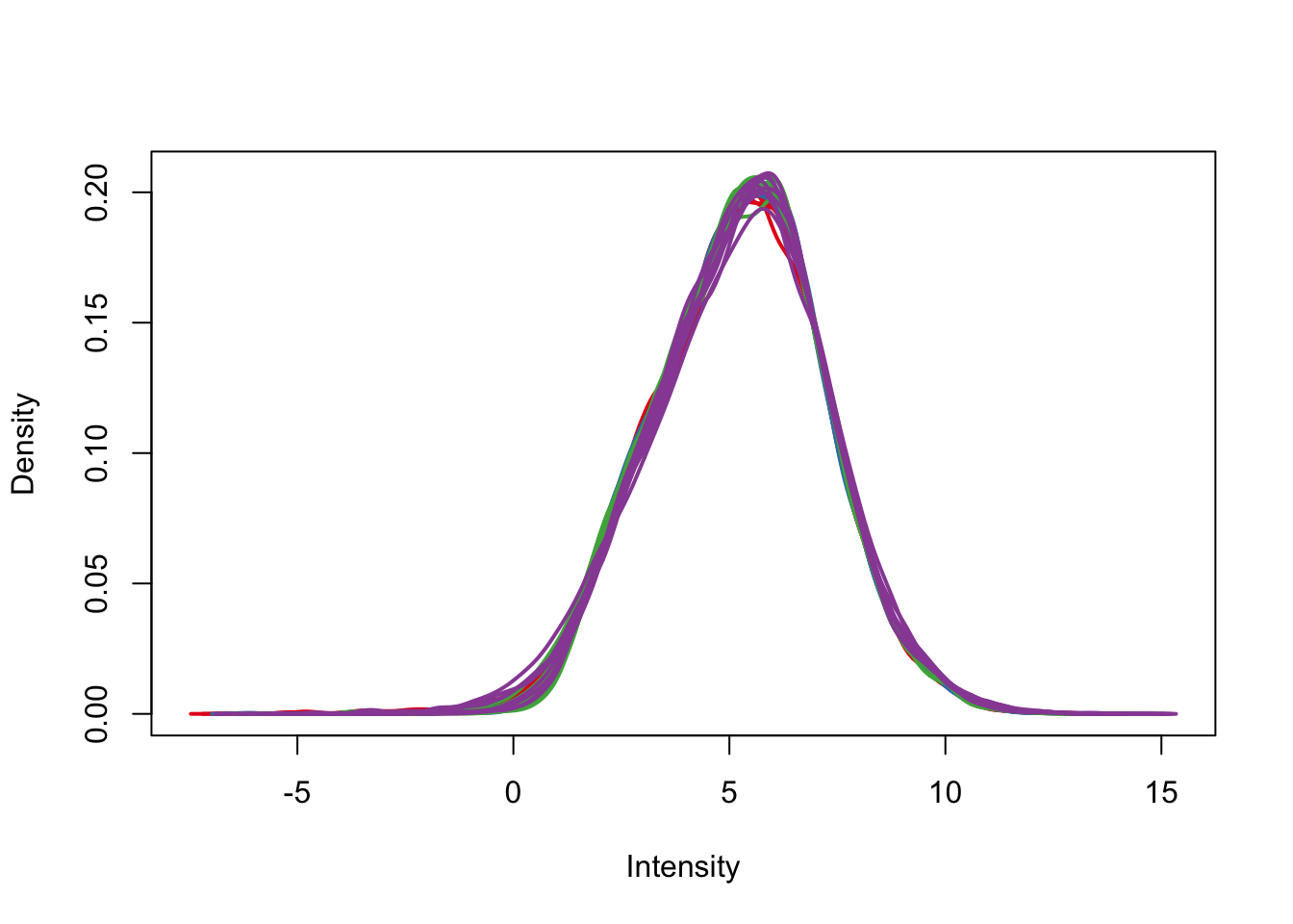
# Run lmFit and eBayes in limma

fit <- lmFit(cpm.voom.corfit , design, block=individual, correlation=corfit.correlation)


# In the contrast matrix, we have the species DE at each day

cm2 <- makeContrasts(HvCday0 = Human, HvCday1 = Human + Human.day1, HvCday2 = Human + Human.day2, HvCday3 = Human + Human.day3, Hday01 = day1 + Human.day1, Hday12 = day2 + Human.day2 - day1 - Human.day1, Hday23 = day3 + Human.day3 - day2 - Human.day2, Cday01 = day1, Cday12 = day2 - day1, Cday23 = day3 - day2, Sig_inter_day1 = Human.day1, Sig_inter_day2 = Human.day2 - Human.day1, Sig_inter_day3 = Human.day3 - Human.day2, levels = design)

# Fit the new model
diff_species <- contrasts.fit(fit, cm2)
fit2 <- eBayes(diff_species)


top3 <- list(HvCday0 =topTable(fit2, coef=1, adjust="BH", number=Inf, sort.by="none"), HvCday1 =topTable(fit2, coef=2, adjust="BH", number=Inf, sort.by="none"),  HvCday2 =topTable(fit2, coef=3, adjust="BH", number=Inf, sort.by="none"),  HvCday3 =topTable(fit2, coef=4, adjust="BH", number=Inf, sort.by="none"), Hday01 =topTable(fit2, coef=5, adjust="BH", number=Inf, sort.by="none"), Hday12 =topTable(fit2, coef=6, adjust="BH", number=Inf, sort.by="none"),  Hday23 =topTable(fit2, coef=7, adjust="BH", number=Inf, sort.by="none"),  Cday01 =topTable(fit2, coef=8, adjust="BH", number=Inf, sort.by="none"), Cday12 =topTable(fit2, coef=9, adjust="BH", number=Inf, sort.by="none"), Cday23 =topTable(fit2, coef=10, adjust="BH", number=Inf, sort.by="none"), Sig_inter_day1 =topTable(fit2, coef=11, adjust="BH", number=Inf, sort.by="none"), Sig_inter_day2 =topTable(fit2, coef=12, adjust="BH", number=Inf, sort.by="none"), Sig_inter_day3 =topTable(fit2, coef=13, adjust="BH", number=Inf, sort.by="none"))

#write.table(fit2, "~/Dropbox/Endoderm TC/Cyclic_loess_norm/unscaled_SD.txt", sep="\t")


# Set FDR level at 5%

FDR_level <- 0.05
#FDR_level <- 0.01


important_columns <- c(1,2,6)

# Find the genes that are DE at Day 0
HvCday0 =topTable(fit2, coef=1, adjust="BH", number=Inf, sort.by="none")
dim(HvCday0[which(HvCday0$adj.P.Val < 0.05), important_columns])
[1] 3205 3HvCday0_adj_pval <- HvCday0[, important_columns]
# Find the genes that are DE at Day 1
HvCday1 =topTable(fit2, coef=2, adjust="BH", number=Inf, sort.by="none")
dim(HvCday1[which(HvCday1$adj.P.Val < 0.05), important_columns])[1] 3024 3HvCday1_adj_pval <- HvCday1[, important_columns]
# Find the genes that are DE at Day 2
HvCday2 =topTable(fit2, coef=3, adjust="BH", number=Inf, sort.by="none")
dim(HvCday2[which(HvCday2$adj.P.Val < 0.05), important_columns]) [1] 3417 3HvCday2_adj_pval <- HvCday2[, important_columns]
# Find the genes that are DE at Day 3
HvCday3 =topTable(fit2, coef=4, adjust="BH", number=Inf, sort.by="none")
dim(HvCday3[which(HvCday3$adj.P.Val < 0.05), important_columns]) [1] 3848 3HvCday3_adj_pval <- HvCday3[, important_columns]
# 3205
# 3024
# 3417
# 3848
important_columns <- c(1,2,6)
# Find the genes that are DE at Day 0
HvCday0 =topTable(fit2, coef=1, adjust="BH", number=Inf, sort.by="none")
dim(HvCday0[which(HvCday0$adj.P.Val < FDR_level), important_columns]) [1] 3205 3HvCday0_adj_pval <- HvCday0[, important_columns]
# Find the genes that are DE at Day 1
HvCday1 =topTable(fit2, coef=2, adjust="BH", number=Inf, sort.by="none")
dim(HvCday1[which(HvCday1$adj.P.Val < FDR_level), important_columns])[1] 3024 3HvCday1_adj_pval <- HvCday1[, important_columns]
# Find the genes that are DE at Day 2
HvCday2 =topTable(fit2, coef=3, adjust="BH", number=Inf, sort.by="none")
dim(HvCday2[which(HvCday2$adj.P.Val < FDR_level), important_columns]) [1] 3417 3HvCday2_adj_pval <- HvCday2[, important_columns]
# Find the genes that are DE at Day 3
HvCday3 =topTable(fit2, coef=4, adjust="BH", number=Inf, sort.by="none")
dim(HvCday3[which(HvCday3$adj.P.Val < FDR_level), important_columns]) [1] 3848 3HvCday3_adj_pval <- HvCday3[, important_columns]
important_columns <- c(1,2,6)
# Find the genes that are DE at Human Day 0 to Day 1
H_day01 =topTable(fit2, coef=5, adjust="BH", number=Inf, sort.by="none")
dim(H_day01[which(H_day01$adj.P.Val < FDR_level), important_columns])[1] 2077 3H_day01 <- H_day01[, important_columns]
# Find the genes that are DE at Human Day 1 to Day 2
H_day12 =topTable(fit2, coef=6, adjust="BH", number=Inf, sort.by="none")
dim(H_day12[which(H_day12$adj.P.Val < FDR_level), important_columns])[1] 2932 3H_day12 <- H_day12[, important_columns]
# Find the genes that are DE at Human Day 2 to Day 3
H_day23 =topTable(fit2, coef=7, adjust="BH", number=Inf, sort.by="none")
dim(H_day23[which(H_day23$adj.P.Val < FDR_level), important_columns])[1] 953 3H_day23 <- H_day23[, important_columns]
# Find the genes that are DE at Chimp Day 0 to Day 1
C_day01 =topTable(fit2, coef=8, adjust="BH", number=Inf, sort.by="none")
dim(C_day01[which(C_day01$adj.P.Val < FDR_level), important_columns])[1] 2875 3C_day01 <- C_day01[, important_columns]
# Find the genes that are DE at Chimp Day 1 to Day 2
C_day12 =topTable(fit2, coef=9, adjust="BH", number=Inf, sort.by="none")
dim(C_day12[which(C_day12$adj.P.Val < FDR_level), important_columns])[1] 4330 3C_day12 <- C_day12[, important_columns]
# Find the genes that are DE at Chimp Day 2 to Day 3
C_day23 =topTable(fit2, coef=10, adjust="BH", number=Inf, sort.by="none")
dim(C_day23[which(C_day23$adj.P.Val < FDR_level), important_columns])[1] 2685 3C_day23 <- C_day23[, important_columns]
# Interactions
# Find the genes with sign interactions Day 1
Sign_day1_inter =topTable(fit2, coef=11, adjust="BH", number=Inf, sort.by="none")
dim(Sign_day1_inter[which(Sign_day1_inter$adj.P.Val < FDR_level), important_columns])[1] 136 3Sign_day1_inter <- Sign_day1_inter[, important_columns]
# Find the genes that are DE at Human Day 1 to Day 2
Sign_day2_inter =topTable(fit2, coef=12, adjust="BH", number=Inf, sort.by="none")
dim(Sign_day2_inter[which(Sign_day2_inter$adj.P.Val < FDR_level), important_columns])[1] 646 3Sign_day2_inter <- Sign_day2_inter[, important_columns]
# Find the genes that are DE at Human Day 2 to Day 3
Sign_day3_inter =topTable(fit2, coef=13, adjust="BH", number=Inf, sort.by="none")
dim(Sign_day3_inter[which(Sign_day3_inter$adj.P.Val < FDR_level), important_columns])[1] 282 3Sign_day3_inter <- Sign_day3_inter[, important_columns]
##################### VENN DIAGRAMS ############################
## DE across species
mylist <- list()
mylist[["DE Day 0"]] <- row.names(top3[[names(top3)[1]]])[top3[[names(top3)[1]]]$adj.P.Val < FDR_level]
mylist[["DE Day 3"]] <- row.names(top3[[names(top3)[4]]])[top3[[names(top3)[4]]]$adj.P.Val < FDR_level]
mylist[["DE Day 1"]] <- row.names(top3[[names(top3)[2]]])[top3[[names(top3)[2]]]$adj.P.Val < FDR_level]
mylist[["DE Day 2"]] <- row.names(top3[[names(top3)[3]]])[top3[[names(top3)[3]]]$adj.P.Val < FDR_level]
# Make as pdf
Four_comp <- venn.diagram(mylist, filename= NULL, main="DE genes between species per day (5% FDR, batch 2)", cex=1.5 , fill = pal[1:4], lty=1, height=2000, width=3000)
pdf(file = "~/Dropbox/Endoderm TC/Tables_Supplement/Supplementary_Figures/SF_4m_DE_by_species_March_13_5FDR_Batch2.pdf")
grid.draw(Four_comp)
dev.off()quartz_off_screen
2 mylist_humans_by_day <- list()
mylist_humans_by_day[["DE Days 0 to 1"]] <- row.names(top3[[names(top3)[5]]])[top3[[names(top3)[5]]]$adj.P.Val < FDR_level]
mylist_humans_by_day[["DE Days 1 to 2"]] <- row.names(top3[[names(top3)[6]]])[top3[[names(top3)[6]]]$adj.P.Val < FDR_level]
mylist_humans_by_day[["DE Days 2 to 3"]] <- row.names(top3[[names(top3)[7]]])[top3[[names(top3)[7]]]$adj.P.Val < FDR_level]
Three_comp_humans <- venn.diagram(mylist_humans_by_day, filename= NULL, main="DE genes across days in humans (1% FDR, batch 2)", cex=1.5 , fill = pal[1:3], lty=1, height=2000, width=3000)
pdf(file = "~/Dropbox/Endoderm TC/Tables_Supplement/Supplementary_Figures/SF_4n_DE_by_day_humans_March_13_5FDR_Batch2.pdf")
grid.draw(Three_comp_humans)
dev.off()quartz_off_screen
2 mylist_chimps_by_day <- list()
mylist_chimps_by_day[["DE Days 0 to 1"]] <- row.names(top3[[names(top3)[8]]])[top3[[names(top3)[8]]]$adj.P.Val < FDR_level]
mylist_chimps_by_day[["DE Days 1 to 2"]] <- row.names(top3[[names(top3)[9]]])[top3[[names(top3)[9]]]$adj.P.Val < FDR_level]
mylist_chimps_by_day[["DE Days 2 to 3"]] <- row.names(top3[[names(top3)[10]]])[top3[[names(top3)[10]]]$adj.P.Val < FDR_level]
Three_comp_chimps <- venn.diagram(mylist_chimps_by_day, filename= NULL, main="DE genes across days in chimpanzees (5% FDR, batch 2)", cex=1.5 , fill = pal[1:3], lty=1, height=2000, width=3000)
pdf(file = "~/Dropbox/Endoderm TC/Tables_Supplement/Supplementary_Figures/SF_4o_DE_by_day_chimps_March_13_5FDR_Batch2.pdf")
grid.draw(Three_comp_chimps)
dev.off()quartz_off_screen
2 mylist_interact <- list()
mylist_interact[["Human x Day 1"]] <- row.names(top3[[names(top3)[11]]])[top3[[names(top3)[11]]]$adj.P.Val < FDR_level]
mylist_interact[["Human x Day 2"]] <- row.names(top3[[names(top3)[12]]])[top3[[names(top3)[12]]]$adj.P.Val < FDR_level]
mylist_interact[["Human x Day 3"]] <- row.names(top3[[names(top3)[13]]])[top3[[names(top3)[13]]]$adj.P.Val < FDR_level]
Sig_interaction <- venn.diagram(mylist_interact, filename= NULL, main="Genes with a significant species-by-day interaction (5% FDR, batch 2)", cex=1.5 , fill = pal[1:3], lty=1, height=2000, width=3000)
pdf(file = "~/Dropbox/Endoderm TC/Tables_Supplement/Supplementary_Figures/SF_4p_Sign_interaction_March_13_5FDR_Batch2.pdf")
grid.draw(Sig_interaction)
dev.off()quartz_off_screen
2 Robustness with respect to the purity samples (supplement)
We have a total of 30 samples with high confidence purity estimates. At Days 0 and 3, we have high confidence purity estimates for 3 human samples and 4 chimp samples. At Days 1 and 2, we have high confidence purity estimates for 4 human and 4 chimp samples.
First we will look at the the DE by species for all samples that we have high confidence purity estimates for.
# Set FDR level at 5%

FDR_level <- 0.05

purity_info <- c(4, 6:7, 9, 11, 13, 15, 17, 20,22,23,25, 27,29,31,33,36,38,39,41,43,45,47,49,54,55,57,59,61,63)

purity_samples <- After_removal_sample_info[purity_info, ]

species <-  purity_samples$Species
day <- as.factor(purity_samples$Day)
individual <- purity_samples$Individual

design <- model.matrix(~ species*day )

colnames(design)[1] <- "Intercept"
colnames(design) <- gsub("specieshuman", "Human", colnames(design))
colnames(design) <- gsub(":", ".", colnames(design))
#colnames(design) <- gsub("batch2", "batch", colnames(design))

# We want a random effect term for individual. As a result, we want to run voom twice. See https://support.bioconductor.org/p/59700/

cpm.voom <- voom(dge_in_cutoff[,purity_info], design, normalize.method="cyclicloess")

corfit <- duplicateCorrelation(cpm.voom, design, block=individual)

corfit.correlation =   corfit$consensus.correlation

cpm.voom.corfit <- voom(dge_in_cutoff[,purity_info], design, plot = TRUE, normalize.method="cyclicloess", block=individual, correlation = corfit.correlation )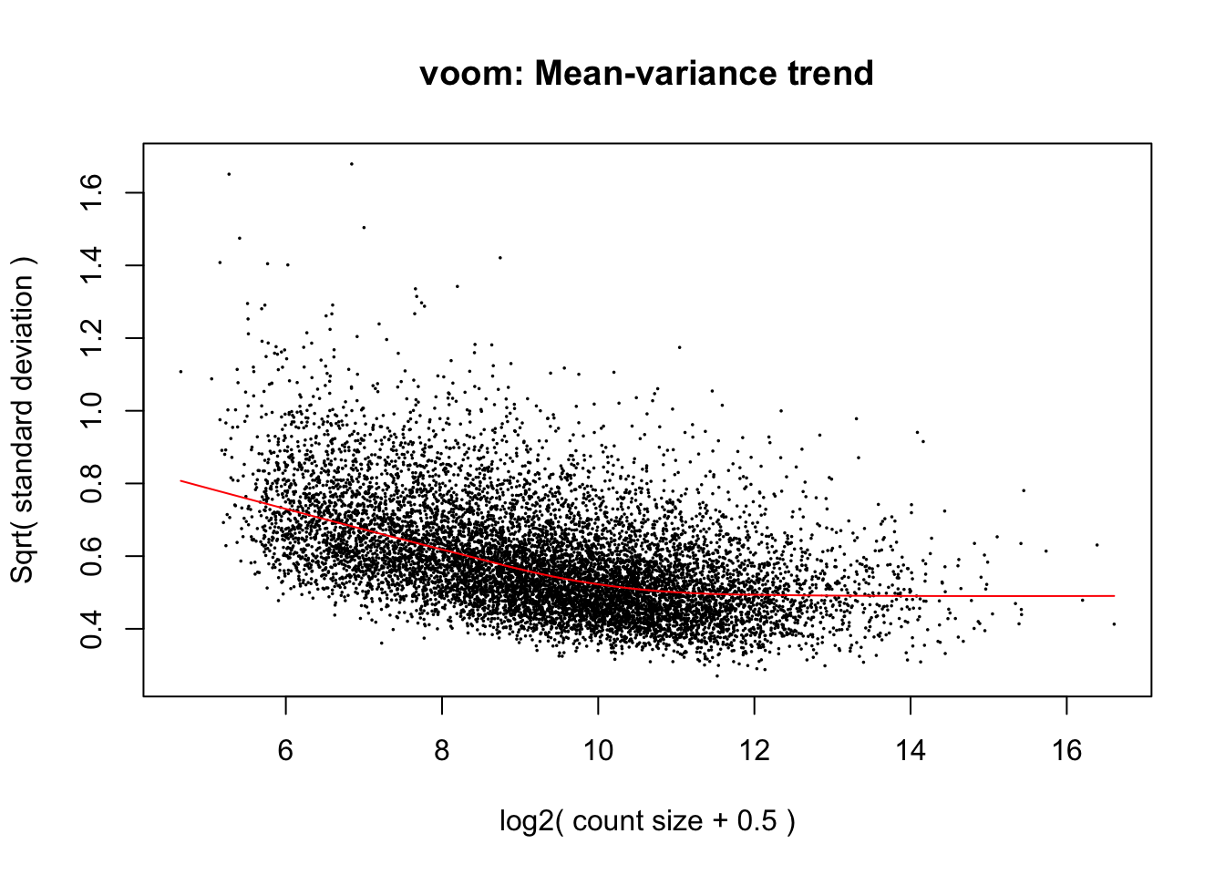
# Plot the density to see shape of the distribution

plotDensities(cpm.voom.corfit, col=pal[as.numeric(day)], legend = F)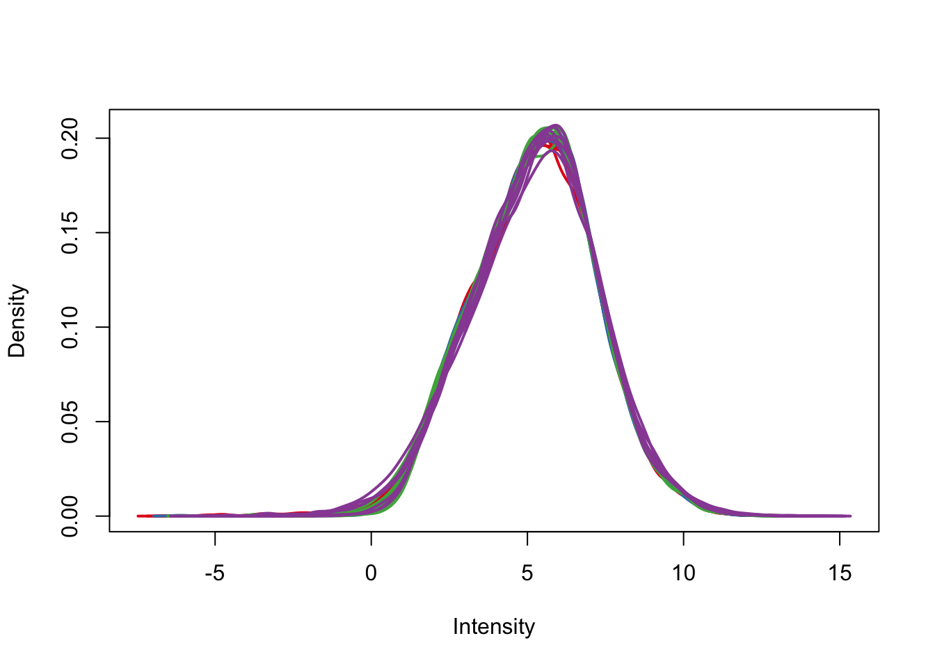
# Run lmFit and eBayes in limma

fit <- lmFit(cpm.voom.corfit , design, block=individual, correlation=corfit.correlation)


# In the contrast matrix, we have the species DE at each day

cm2 <- makeContrasts(HvCday0 = Human, HvCday1 = Human + Human.day1, HvCday2 = Human + Human.day2, HvCday3 = Human + Human.day3, Hday01 = day1 + Human.day1, Hday12 = day2 + Human.day2 - day1 - Human.day1, Hday23 = day3 + Human.day3 - day2 - Human.day2, Cday01 = day1, Cday12 = day2 - day1, Cday23 = day3 - day2, Sig_inter_day1 = Human.day1, Sig_inter_day2 = Human.day2 - Human.day1, Sig_inter_day3 = Human.day3 - Human.day2, levels = design)

# Fit the new model
diff_species <- contrasts.fit(fit, cm2)
fit2 <- eBayes(diff_species)


top3 <- list(HvCday0 =topTable(fit2, coef=1, adjust="BH", number=Inf, sort.by="none"), HvCday1 =topTable(fit2, coef=2, adjust="BH", number=Inf, sort.by="none"),  HvCday2 =topTable(fit2, coef=3, adjust="BH", number=Inf, sort.by="none"),  HvCday3 =topTable(fit2, coef=4, adjust="BH", number=Inf, sort.by="none"), Hday01 =topTable(fit2, coef=5, adjust="BH", number=Inf, sort.by="none"), Hday12 =topTable(fit2, coef=6, adjust="BH", number=Inf, sort.by="none"),  Hday23 =topTable(fit2, coef=7, adjust="BH", number=Inf, sort.by="none"),  Cday01 =topTable(fit2, coef=8, adjust="BH", number=Inf, sort.by="none"), Cday12 =topTable(fit2, coef=9, adjust="BH", number=Inf, sort.by="none"), Cday23 =topTable(fit2, coef=10, adjust="BH", number=Inf, sort.by="none"), Sig_inter_day1 =topTable(fit2, coef=11, adjust="BH", number=Inf, sort.by="none"), Sig_inter_day2 =topTable(fit2, coef=12, adjust="BH", number=Inf, sort.by="none"), Sig_inter_day3 =topTable(fit2, coef=13, adjust="BH", number=Inf, sort.by="none"))

#write.table(fit2, "~/Dropbox/Endoderm TC/Cyclic_loess_norm/unscaled_SD.txt", sep="\t")


# Set FDR level at 5%

FDR_level <- 0.05
#FDR_level <- 0.01


important_columns <- c(1,2,6)

# Find the genes that are DE at Day 0
HvCday0 =topTable(fit2, coef=1, adjust="BH", number=Inf, sort.by="none")
dim(HvCday0[which(HvCday0$adj.P.Val < 0.05), important_columns])
[1] 3230 3HvCday0_adj_pval <- HvCday0[, important_columns]
# Find the genes that are DE at Day 1
HvCday1 =topTable(fit2, coef=2, adjust="BH", number=Inf, sort.by="none")
dim(HvCday1[which(HvCday1$adj.P.Val < 0.05), important_columns])[1] 3059 3HvCday1_adj_pval <- HvCday1[, important_columns]
# Find the genes that are DE at Day 2
HvCday2 =topTable(fit2, coef=3, adjust="BH", number=Inf, sort.by="none")
dim(HvCday2[which(HvCday2$adj.P.Val < 0.05), important_columns]) [1] 3466 3HvCday2_adj_pval <- HvCday2[, important_columns]
# Find the genes that are DE at Day 3
HvCday3 =topTable(fit2, coef=4, adjust="BH", number=Inf, sort.by="none")
dim(HvCday3[which(HvCday3$adj.P.Val < 0.05), important_columns]) [1] 3551 3HvCday3_adj_pval <- HvCday3[, important_columns]
# 3230
# 3059
# 3466
# 3551
##################### VENN DIAGRAMS ############################
## DE across species
mylist <- list()
mylist[["DE Day 0"]] <- row.names(top3[[names(top3)[1]]])[top3[[names(top3)[1]]]$adj.P.Val < FDR_level]
mylist[["DE Day 3"]] <- row.names(top3[[names(top3)[4]]])[top3[[names(top3)[4]]]$adj.P.Val < FDR_level]
mylist[["DE Day 1"]] <- row.names(top3[[names(top3)[2]]])[top3[[names(top3)[2]]]$adj.P.Val < FDR_level]
mylist[["DE Day 2"]] <- row.names(top3[[names(top3)[3]]])[top3[[names(top3)[3]]]$adj.P.Val < FDR_level]
# Make as pdf
Four_comp <- venn.diagram(mylist, filename= NULL, main="DE genes between species per day (5% FDR, batch 2)", cex=1.5 , fill = pal[1:4], lty=1, height=2000, width=3000)
pdf(file = "~/Dropbox/Endoderm TC/Tables_Supplement/Supplementary_Figures/SF_4q_DE_by_species_March_13_5FDR_All_high_conf_purity.pdf")
grid.draw(Four_comp)
dev.off()quartz_off_screen
2 Now, we can subset and compare 3 humans to 3 chimps that have the highest confidence purity estimates.
# Set FDR level at 5%

FDR_level <- 0.05

purity_info <- c(4, 6:7, 11, 13, 15, 17, 22, 23, 27, 29, 31,33,36, 38, 41,43, 47, 49,54, 55, 59,61,63)

purity_samples <- After_removal_sample_info[purity_info, ]

species <-  purity_samples$Species
day <- as.factor(purity_samples$Day)
individual <- purity_samples$Individual

design <- model.matrix(~ species*day )

colnames(design)[1] <- "Intercept"
colnames(design) <- gsub("specieshuman", "Human", colnames(design))
colnames(design) <- gsub(":", ".", colnames(design))
#colnames(design) <- gsub("batch2", "batch", colnames(design))

# We want a random effect term for individual. As a result, we want to run voom twice. See https://support.bioconductor.org/p/59700/

cpm.voom <- voom(dge_in_cutoff[,purity_info], design, normalize.method="cyclicloess")

corfit <- duplicateCorrelation(cpm.voom, design, block=individual)

corfit.correlation =   corfit$consensus.correlation

cpm.voom.corfit <- voom(dge_in_cutoff[,purity_info], design, plot = TRUE, normalize.method="cyclicloess", block=individual, correlation = corfit.correlation )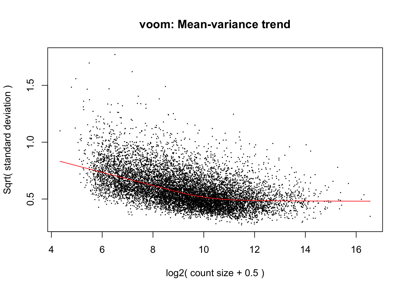
# Plot the density to see shape of the distribution

plotDensities(cpm.voom.corfit, col=pal[as.numeric(day)], legend = F)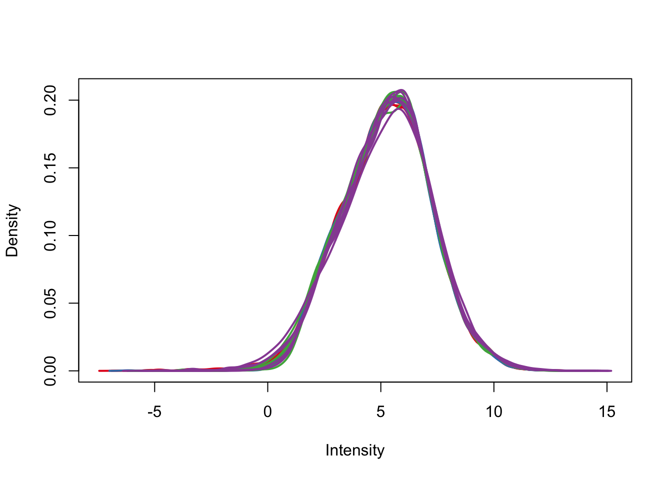
# Run lmFit and eBayes in limma

fit <- lmFit(cpm.voom.corfit , design, block=individual, correlation=corfit.correlation)


# In the contrast matrix, we have the species DE at each day

cm2 <- makeContrasts(HvCday0 = Human, HvCday1 = Human + Human.day1, HvCday2 = Human + Human.day2, HvCday3 = Human + Human.day3, Hday01 = day1 + Human.day1, Hday12 = day2 + Human.day2 - day1 - Human.day1, Hday23 = day3 + Human.day3 - day2 - Human.day2, Cday01 = day1, Cday12 = day2 - day1, Cday23 = day3 - day2, Sig_inter_day1 = Human.day1, Sig_inter_day2 = Human.day2 - Human.day1, Sig_inter_day3 = Human.day3 - Human.day2, levels = design)

# Fit the new model
diff_species <- contrasts.fit(fit, cm2)
fit2 <- eBayes(diff_species)


top3 <- list(HvCday0 =topTable(fit2, coef=1, adjust="BH", number=Inf, sort.by="none"), HvCday1 =topTable(fit2, coef=2, adjust="BH", number=Inf, sort.by="none"),  HvCday2 =topTable(fit2, coef=3, adjust="BH", number=Inf, sort.by="none"),  HvCday3 =topTable(fit2, coef=4, adjust="BH", number=Inf, sort.by="none"), Hday01 =topTable(fit2, coef=5, adjust="BH", number=Inf, sort.by="none"), Hday12 =topTable(fit2, coef=6, adjust="BH", number=Inf, sort.by="none"),  Hday23 =topTable(fit2, coef=7, adjust="BH", number=Inf, sort.by="none"),  Cday01 =topTable(fit2, coef=8, adjust="BH", number=Inf, sort.by="none"), Cday12 =topTable(fit2, coef=9, adjust="BH", number=Inf, sort.by="none"), Cday23 =topTable(fit2, coef=10, adjust="BH", number=Inf, sort.by="none"), Sig_inter_day1 =topTable(fit2, coef=11, adjust="BH", number=Inf, sort.by="none"), Sig_inter_day2 =topTable(fit2, coef=12, adjust="BH", number=Inf, sort.by="none"), Sig_inter_day3 =topTable(fit2, coef=13, adjust="BH", number=Inf, sort.by="none"))

#write.table(fit2, "~/Dropbox/Endoderm TC/Cyclic_loess_norm/unscaled_SD.txt", sep="\t")


# Set FDR level at 5%

FDR_level <- 0.05
#FDR_level <- 0.01


important_columns <- c(1,2,6)

# Find the genes that are DE at Day 0
HvCday0 =topTable(fit2, coef=1, adjust="BH", number=Inf, sort.by="none")
dim(HvCday0[which(HvCday0$adj.P.Val < 0.05), important_columns])
[1] 2290 3HvCday0_adj_pval <- HvCday0[, important_columns]
# Find the genes that are DE at Day 1
HvCday1 =topTable(fit2, coef=2, adjust="BH", number=Inf, sort.by="none")
dim(HvCday1[which(HvCday1$adj.P.Val < 0.05), important_columns])[1] 2242 3HvCday1_adj_pval <- HvCday1[, important_columns]
# Find the genes that are DE at Day 2
HvCday2 =topTable(fit2, coef=3, adjust="BH", number=Inf, sort.by="none")
dim(HvCday2[which(HvCday2$adj.P.Val < 0.05), important_columns]) [1] 2694 3HvCday2_adj_pval <- HvCday2[, important_columns]
# Find the genes that are DE at Day 3
HvCday3 =topTable(fit2, coef=4, adjust="BH", number=Inf, sort.by="none")
dim(HvCday3[which(HvCday3$adj.P.Val < 0.05), important_columns]) [1] 2829 3HvCday3_adj_pval <- HvCday3[, important_columns]
# 2290
# 2242
# 2694
# 2829
##################### VENN DIAGRAMS ############################
## DE across species
mylist <- list()
mylist[["DE Day 0"]] <- row.names(top3[[names(top3)[1]]])[top3[[names(top3)[1]]]$adj.P.Val < FDR_level]
mylist[["DE Day 3"]] <- row.names(top3[[names(top3)[4]]])[top3[[names(top3)[4]]]$adj.P.Val < FDR_level]
mylist[["DE Day 1"]] <- row.names(top3[[names(top3)[2]]])[top3[[names(top3)[2]]]$adj.P.Val < FDR_level]
mylist[["DE Day 2"]] <- row.names(top3[[names(top3)[3]]])[top3[[names(top3)[3]]]$adj.P.Val < FDR_level]
# Make as pdf
Four_comp <- venn.diagram(mylist, filename= NULL, main="DE genes between species per day (5% FDR, 3 highest purity/group)", cex=1.5 , fill = pal[1:4], lty=1, height=2000, width=3000)
pdf(file = "~/Dropbox/Endoderm TC/Tables_Supplement/Supplementary_Figures/SF_4r_DE_by_species_March_13_5FDR_3_high_conf_purity.pdf")
grid.draw(Four_comp)
dev.off()quartz_off_screen
2 Now, we can subset and compare 3 humans to 3 chimps that have the lowest high confidence purity estimates.
# Set FDR level at 5%

FDR_level <- 0.05

purity_info <- c(4, 6:7, 9, 13, 15, 17, 20, 22, 25, 27, 29, 36,38, 39, 43,45, 47, 49,54, 55, 57,61,63)

purity_samples <- After_removal_sample_info[purity_info, ]

species <-  purity_samples$Species
day <- as.factor(purity_samples$Day)
individual <- purity_samples$Individual

design <- model.matrix(~ species*day )

colnames(design)[1] <- "Intercept"
colnames(design) <- gsub("specieshuman", "Human", colnames(design))
colnames(design) <- gsub(":", ".", colnames(design))
#colnames(design) <- gsub("batch2", "batch", colnames(design))

# We want a random effect term for individual. As a result, we want to run voom twice. See https://support.bioconductor.org/p/59700/

cpm.voom <- voom(dge_in_cutoff[,purity_info], design, normalize.method="cyclicloess")

corfit <- duplicateCorrelation(cpm.voom, design, block=individual)

corfit.correlation =   corfit$consensus.correlation

cpm.voom.corfit <- voom(dge_in_cutoff[,purity_info], design, plot = TRUE, normalize.method="cyclicloess", block=individual, correlation = corfit.correlation )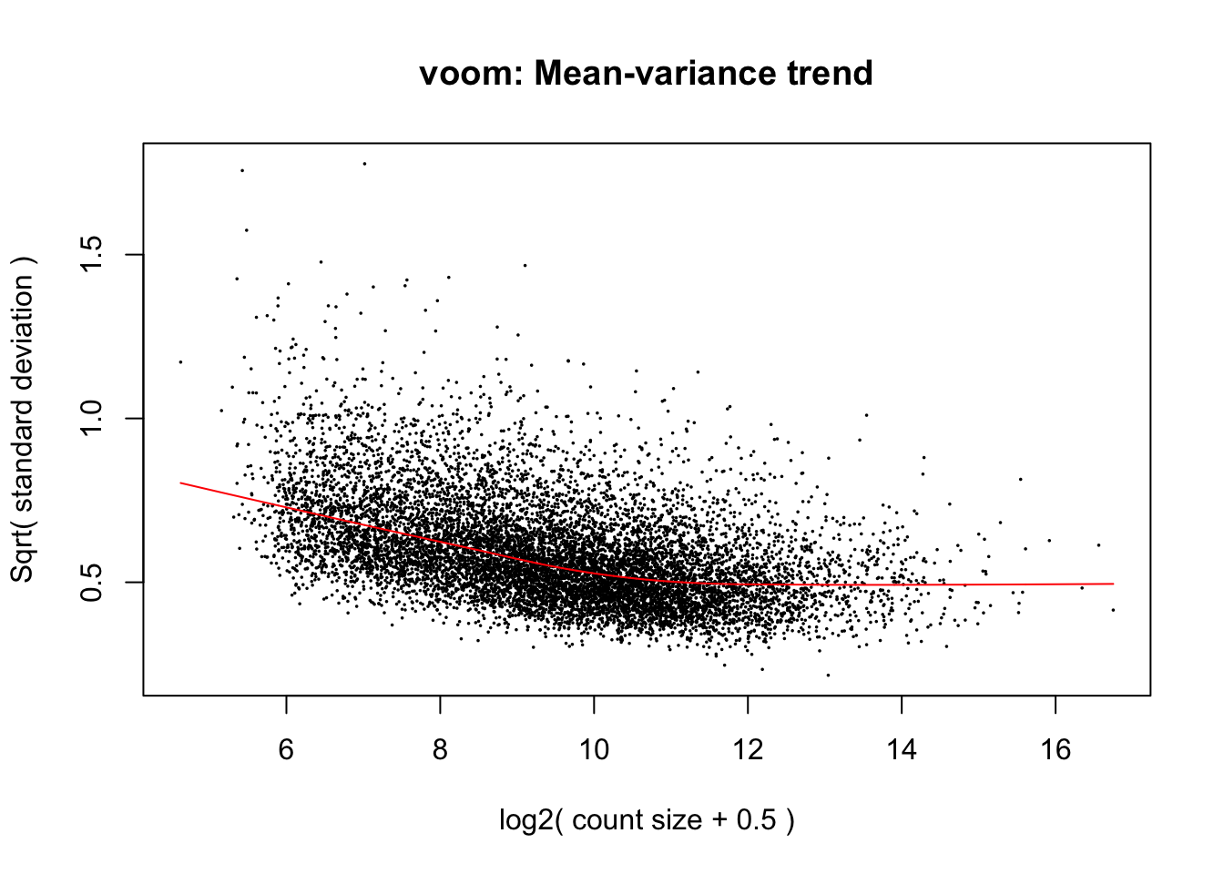
# Plot the density to see shape of the distribution

plotDensities(cpm.voom.corfit, col=pal[as.numeric(day)], legend = F)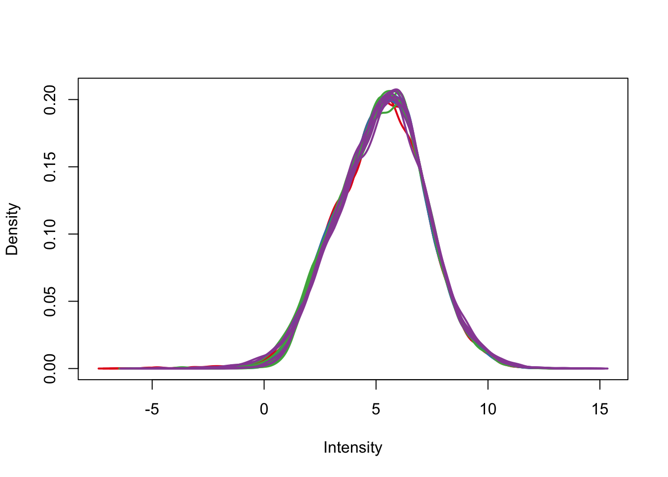
# Run lmFit and eBayes in limma

fit <- lmFit(cpm.voom.corfit , design, block=individual, correlation=corfit.correlation)


# In the contrast matrix, we have the species DE at each day

cm2 <- makeContrasts(HvCday0 = Human, HvCday1 = Human + Human.day1, HvCday2 = Human + Human.day2, HvCday3 = Human + Human.day3, Hday01 = day1 + Human.day1, Hday12 = day2 + Human.day2 - day1 - Human.day1, Hday23 = day3 + Human.day3 - day2 - Human.day2, Cday01 = day1, Cday12 = day2 - day1, Cday23 = day3 - day2, Sig_inter_day1 = Human.day1, Sig_inter_day2 = Human.day2 - Human.day1, Sig_inter_day3 = Human.day3 - Human.day2, levels = design)

# Fit the new model
diff_species <- contrasts.fit(fit, cm2)
fit2 <- eBayes(diff_species)


top3 <- list(HvCday0 =topTable(fit2, coef=1, adjust="BH", number=Inf, sort.by="none"), HvCday1 =topTable(fit2, coef=2, adjust="BH", number=Inf, sort.by="none"),  HvCday2 =topTable(fit2, coef=3, adjust="BH", number=Inf, sort.by="none"),  HvCday3 =topTable(fit2, coef=4, adjust="BH", number=Inf, sort.by="none"), Hday01 =topTable(fit2, coef=5, adjust="BH", number=Inf, sort.by="none"), Hday12 =topTable(fit2, coef=6, adjust="BH", number=Inf, sort.by="none"),  Hday23 =topTable(fit2, coef=7, adjust="BH", number=Inf, sort.by="none"),  Cday01 =topTable(fit2, coef=8, adjust="BH", number=Inf, sort.by="none"), Cday12 =topTable(fit2, coef=9, adjust="BH", number=Inf, sort.by="none"), Cday23 =topTable(fit2, coef=10, adjust="BH", number=Inf, sort.by="none"), Sig_inter_day1 =topTable(fit2, coef=11, adjust="BH", number=Inf, sort.by="none"), Sig_inter_day2 =topTable(fit2, coef=12, adjust="BH", number=Inf, sort.by="none"), Sig_inter_day3 =topTable(fit2, coef=13, adjust="BH", number=Inf, sort.by="none"))

#write.table(fit2, "~/Dropbox/Endoderm TC/Cyclic_loess_norm/unscaled_SD.txt", sep="\t")


# Set FDR level at 5%

FDR_level <- 0.05
#FDR_level <- 0.01


important_columns <- c(1,2,6)

# Find the genes that are DE at Day 0
HvCday0 =topTable(fit2, coef=1, adjust="BH", number=Inf, sort.by="none")
dim(HvCday0[which(HvCday0$adj.P.Val < 0.05), important_columns])
[1] 2894 3HvCday0_adj_pval <- HvCday0[, important_columns]
# Find the genes that are DE at Day 1
HvCday1 =topTable(fit2, coef=2, adjust="BH", number=Inf, sort.by="none")
dim(HvCday1[which(HvCday1$adj.P.Val < 0.05), important_columns])[1] 2375 3HvCday1_adj_pval <- HvCday1[, important_columns]
# Find the genes that are DE at Day 2
HvCday2 =topTable(fit2, coef=3, adjust="BH", number=Inf, sort.by="none")
dim(HvCday2[which(HvCday2$adj.P.Val < 0.05), important_columns]) [1] 2838 3HvCday2_adj_pval <- HvCday2[, important_columns]
# Find the genes that are DE at Day 3
HvCday3 =topTable(fit2, coef=4, adjust="BH", number=Inf, sort.by="none")
dim(HvCday3[which(HvCday3$adj.P.Val < 0.05), important_columns]) [1] 3034 3HvCday3_adj_pval <- HvCday3[, important_columns]
# 2894
# 2375
# 2838
# 3034
##################### VENN DIAGRAMS ############################
## DE across species
mylist <- list()
mylist[["DE Day 0"]] <- row.names(top3[[names(top3)[1]]])[top3[[names(top3)[1]]]$adj.P.Val < FDR_level]
mylist[["DE Day 3"]] <- row.names(top3[[names(top3)[4]]])[top3[[names(top3)[4]]]$adj.P.Val < FDR_level]
mylist[["DE Day 1"]] <- row.names(top3[[names(top3)[2]]])[top3[[names(top3)[2]]]$adj.P.Val < FDR_level]
mylist[["DE Day 2"]] <- row.names(top3[[names(top3)[3]]])[top3[[names(top3)[3]]]$adj.P.Val < FDR_level]
# Make as pdf
Four_comp <- venn.diagram(mylist, filename= NULL, main="DE genes between species per day (5% FDR, 3 lowest purity/group)", cex=1.5 , fill = pal[1:4], lty=1, height=2000, width=3000)
pdf(file = "~/Dropbox/Endoderm TC/Tables_Supplement/Supplementary_Figures/SF_4s_DE_by_species_March_13_5FDR_3_low_conf_purity.pdf")
grid.draw(Four_comp)
dev.off()quartz_off_screen
2 Final global correction (supplement)
species <- c("H", "H","H","H","H","H","H", "C", "C","C","C","C","C","C","C","H","H","H","H","H","H","H","H",  "C", "C","C","C","C","C","C","C", "H","H","H","H","H","H","H","H",  "C", "C","C","C","C","C","C","C", "H","H","H","H","H","H","H","H",  "C", "C","C","C","C","C","C","C")

day <- c("0", "0","0","0","0","0","0", "0", "0", "0","0","0","0","0", "0","1","1","1","1","1","1","1","1", "1","1","1","1","1","1","1","1",  "2", "2","2","2","2","2","2","2","2", "2","2","2","2","2","2","2",  "3", "3","3","3","3","3","3","3",  "3", "3","3","3","3","3","3", "3")

design <- model.matrix(~ species*day )

colnames(design)[1] <- "Intercept"
colnames(design) <- gsub("speciesH", "Human", colnames(design))
colnames(design) <- gsub(":", ".", colnames(design))
#colnames(design) <- gsub("batch2", "batch", colnames(design))

individual <- After_removal_sample_info$Individual

# We want a random effect term for individual. As a result, we want to run voom twice. See https://support.bioconductor.org/p/59700/

cpm.voom <- voom(dge_in_cutoff, design, normalize.method="cyclicloess")

corfit.correlation = corfit$consensus.correlation

cpm.voom.corfit <- voom(dge_in_cutoff, design, plot = TRUE, normalize.method="cyclicloess", block=individual, correlation = corfit.correlation )
# Plot the density to see shape of the distribution

plotDensities(cpm.voom.corfit, col=pal[as.numeric(day)], legend = F)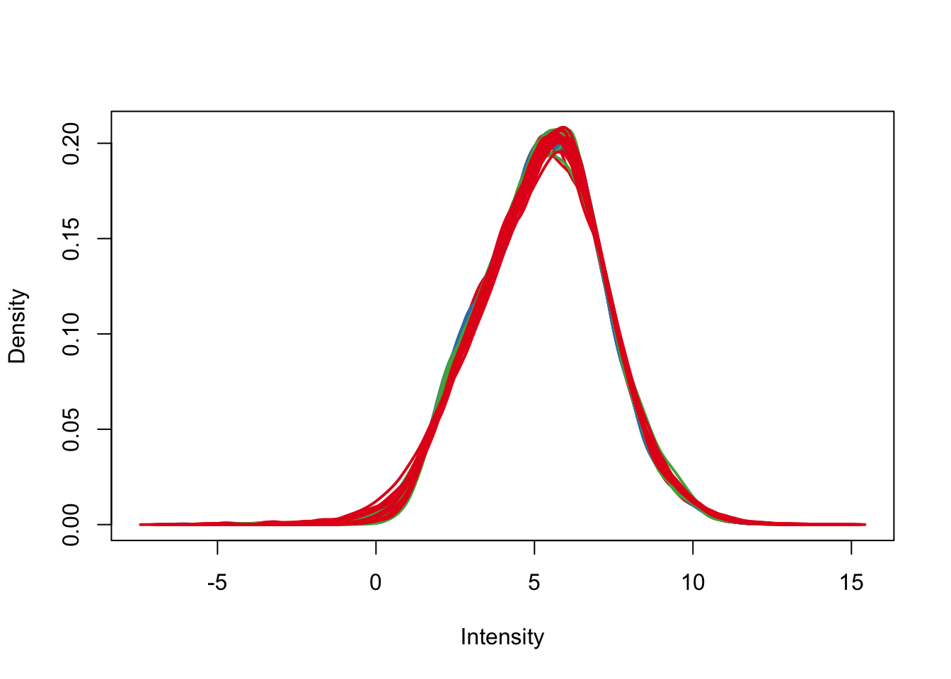
# Run lmFit and eBayes in limma

fit <- lmFit(cpm.voom.corfit , design, block=individual, correlation=corfit.correlation)


# In the contrast matrix, we have the species DE at each day

cm2 <- makeContrasts(HvCday0 = Human, HvCday1 = Human + Human.day1, HvCday2 = Human + Human.day2, HvCday3 = Human + Human.day3, Hday01 = day1 + Human.day1, Hday12 = day2 + Human.day2 - day1 - Human.day1, Hday23 = day3 + Human.day3 - day2 - Human.day2, Cday01 = day1, Cday12 = day2 - day1, Cday23 = day3 - day2, Sig_inter_day1 = Human.day1, Sig_inter_day2 = Human.day2 - Human.day1, Sig_inter_day3 = Human.day3 - Human.day2, levels = design)

# Fit the new model
diff_species <- contrasts.fit(fit, cm2)
fit2 <- eBayes(diff_species)


top3 <- list(HvCday0 =topTable(fit2, coef=1, adjust="BH", number=Inf, sort.by="none"), HvCday1 =topTable(fit2, coef=2, adjust="BH", number=Inf, sort.by="none"),  HvCday2 =topTable(fit2, coef=3, adjust="BH", number=Inf, sort.by="none"),  HvCday3 =topTable(fit2, coef=4, adjust="BH", number=Inf, sort.by="none"), Hday01 =topTable(fit2, coef=5, adjust="BH", number=Inf, sort.by="none"), Hday12 =topTable(fit2, coef=6, adjust="BH", number=Inf, sort.by="none"),  Hday23 =topTable(fit2, coef=7, adjust="BH", number=Inf, sort.by="none"),  Cday01 =topTable(fit2, coef=8, adjust="BH", number=Inf, sort.by="none"), Cday12 =topTable(fit2, coef=9, adjust="BH", number=Inf, sort.by="none"), Cday23 =topTable(fit2, coef=10, adjust="BH", number=Inf, sort.by="none"), Sig_inter_day1 =topTable(fit2, coef=11, adjust="BH", number=Inf, sort.by="none"), Sig_inter_day2 =topTable(fit2, coef=12, adjust="BH", number=Inf, sort.by="none"), Sig_inter_day3 =topTable(fit2, coef=13, adjust="BH", number=Inf, sort.by="none"))

# Compare separate versus global

separate_rank <- decideTests(fit2, method = "separate", adjust.method = "BH")
summary(decideTests(fit2, method = "separate", adjust.method = "BH", p.value = 0.05))
HvCday0 HvCday1 HvCday2 HvCday3 Hday01 Hday12 Hday23 Cday01 Cday12
-1 1711 1698 1761 1980 1717 2315 872 1780 2451
0 6932 7017 6740 6369 6846 5734 8604 6685 5607
1 1661 1589 1803 1955 1741 2255 828 1839 2246
Cday23 Sig_inter_day1 Sig_inter_day2 Sig_inter_day3
-1 1925 195 322 249
0 6350 9935 9633 9807
1 2029 174 349 248global_rank <- decideTests(fit2, method = "global", adjust.method = "BH")
summary(decideTests(fit2, method = "global", adjust.method = "BH", p.value = 0.05)) HvCday0 HvCday1 HvCday2 HvCday3 Hday01 Hday12 Hday23 Cday01 Cday12
-1 1659 1648 1689 1849 1671 2138 1023 1710 2269
0 7034 7105 6872 6603 6946 6065 8296 6823 5941
1 1611 1551 1743 1852 1687 2101 985 1771 2094
Cday23 Sig_inter_day1 Sig_inter_day2 Sig_inter_day3
-1 1843 408 542 537
0 6559 9520 9153 9209
1 1902 376 609 558# Set FDR level at 5%
FDR_level <- 0.05
#FDR_level <- 0.01
important_columns <- c(1,2,6)
# Find the genes that are DE at Day 0
HvCday0 <- row.names(as.data.frame(which(global_rank[,1] !=0) ))
# Find the genes that are DE at Day 1
HvCday1 <- row.names(as.data.frame(which(global_rank[,2] !=0) ))
# Find the genes that are DE at Day 2
HvCday2 <- row.names(as.data.frame(which(global_rank[,3] !=0) ))
# Find the genes that are DE at Day 3
HvCday3 <- row.names(as.data.frame(which(global_rank[,4] !=0) ))
length(HvCday0)[1] 3270# 3153
length(HvCday1)[1] 3199# 3098
length(HvCday2)[1] 3432# 3336
length(HvCday3)[1] 3701# 3597
write.table(HvCday0, "~/Dropbox/Endoderm TC/DE Analysis_Pairwise/Final_global/HvC_day0_sign_p_0.05", sep="\t")
write.table(HvCday1, "~/Dropbox/Endoderm TC/DE Analysis_Pairwise/Final_global/HvC_day1_sign_p_0.05", sep="\t")
write.table(HvCday2, "~/Dropbox/Endoderm TC/DE Analysis_Pairwise/Final_global/HvC_day2_sign_p_0.05", sep="\t")
write.table(HvCday3, "~/Dropbox/Endoderm TC/DE Analysis_Pairwise/Final_global/HvC_day3_sign_p_0.05", sep="\t")
important_columns <- c(1,2,6)
# Find the genes that are DE at Human Day 0 to Day 1
H_day01 = row.names(as.data.frame(which(global_rank[,5] !=0) ))
# Find the genes that are DE at Human Day 1 to Day 2
H_day12 = row.names(as.data.frame(which(global_rank[,6] !=0) ))
# Find the genes that are DE at Human Day 2 to Day 3
H_day23 = row.names(as.data.frame(which(global_rank[,7] !=0) ))
# Find the genes that are DE at Chimp Day 0 to Day 1
C_day01 = row.names(as.data.frame(which(global_rank[,8] !=0) ))
# Find the genes that are DE at Chimp Day 1 to Day 2
C_day12 = row.names(as.data.frame(which(global_rank[,9] !=0) ))
# Find the genes that are DE at Chimp Day 2 to Day 3
C_day23 = row.names(as.data.frame(which(global_rank[,10] !=0) ))
# Make a table of the sections
write.table(H_day01, "~/Dropbox/Endoderm TC/DE Analysis_Pairwise/Final_global/H_day01_sign_p_0.05.txt", sep="\t")
write.table(H_day12, "~/Dropbox/Endoderm TC/DE Analysis_Pairwise/Final_global/H_day12_sign_p_0.05", sep="\t")
write.table(H_day23, "~/Dropbox/Endoderm TC/DE Analysis_Pairwise/Final_global/H_day12_sign_p_0.05.txt", sep="\t")
write.table(C_day01, "~/Dropbox/Endoderm TC/DE Analysis_Pairwise/Final_global/C_day01_sign_p_0.05.txt", sep="\t")
write.table(C_day12, "~/Dropbox/Endoderm TC/DE Analysis_Pairwise/Final_global/C_day12_sign_p_0.05.txt", sep="\t")
write.table(C_day23, "~/Dropbox/Endoderm TC/DE Analysis_Pairwise/Final_global/C_day23_sign_p_0.05.txt", sep="\t")
# Interactions
# Find the genes with sign interactions Day 1
Sign_day1_inter = row.names(as.data.frame(which(global_rank[,11] !=0) ))
# Find the genes that are DE at Human Day 1 to Day 2
Sign_day2_inter = row.names(as.data.frame(which(global_rank[,12] !=0) ))
# Find the genes that are DE at Human Day 2 to Day 3
Sign_day3_inter = row.names(as.data.frame(which(global_rank[,13] !=0) ))
# Make a table of the sections
write.table(Sign_day1_inter, "~/Dropbox/Endoderm TC/DE Analysis_Pairwise/Final_global/H_day1_interact_sign_p_0.05.txt", sep="\t")
write.table(Sign_day2_inter, "~/Dropbox/Endoderm TC/DE Analysis_Pairwise/Final_global/H_day2_interact_sign_p_0.05.txt", sep="\t")
write.table(Sign_day3_inter, "~/Dropbox/Endoderm TC/DE Analysis_Pairwise/Final_global/H_day3_interact_sign_p_0.05.txt", sep="\t")
##################### VENN DIAGRAMS ############################
## DE across species
mylist <- list()
mylist[["DE Day 0"]] <- HvCday0
mylist[["DE Day 3"]] <- HvCday3
mylist[["DE Day 1"]] <- HvCday1
mylist[["DE Day 2"]] <- HvCday2
# Make as pdf
Four_comp <- venn.diagram(mylist, filename= NULL, main="DE genes between species per day (5% FDR, global correction)", cex=1.5 , fill = pal[1:4], lty=1, height=2000, width=3000)
pdf(file = "~/Dropbox/Endoderm TC/Tables_Supplement/Supplementary_Figures/SF_4t_DE_by_species_March_13_5FDR_global_correction.pdf")
grid.draw(Four_comp)
dev.off()quartz_off_screen
2 mylist_humans_by_day <- list()
mylist_humans_by_day[["DE Days 0 to 1"]] <- H_day01
mylist_humans_by_day[["DE Days 1 to 2"]] <- H_day12
mylist_humans_by_day[["DE Days 2 to 3"]] <- H_day23
Three_comp_humans <- venn.diagram(mylist_humans_by_day, filename= NULL, main="DE genes across days in humans (5% FDR, global correction)", cex=1.5 , fill = pal[1:3], lty=1, height=2000, width=3000)
pdf(file = "~/Dropbox/Endoderm TC/Tables_Supplement/Supplementary_Figures/SF_4v_DE_by_day_human_March_13_5FDR_global_correction.pdf")
grid.draw(Three_comp_humans)
dev.off()quartz_off_screen
2 mylist_chimps_by_day <- list()
mylist_chimps_by_day[["DE Days 0 to 1"]] <- C_day01
mylist_chimps_by_day[["DE Days 1 to 2"]] <- C_day12
mylist_chimps_by_day[["DE Days 2 to 3"]] <- C_day23
Three_comp_chimps <- venn.diagram(mylist_chimps_by_day, filename= NULL, main="DE genes across days in chimpanzees (5% FDR, global correction)", cex=1.5 , fill = pal[1:3], lty=1, height=2000, width=3000)
pdf(file = "~/Dropbox/Endoderm TC/Tables_Supplement/Supplementary_Figures/SF_4w_DE_by_day_chimp_March_13_5FDR_global_correction.pdf")
grid.draw(Three_comp_chimps)
dev.off()quartz_off_screen
2 mylist_interact <- list()
mylist_interact[["Human x Day 1"]] <- Sign_day1_inter
mylist_interact[["Human x Day 2"]] <- Sign_day2_inter
mylist_interact[["Human x Day 3"]] <- Sign_day3_inter
Sig_interaction <- venn.diagram(mylist_interact, filename= NULL, main="Genes with a significant species-by-day interaction (5% FDR, global correction)", cex=1.5 , fill = pal[1:3], lty=1, height=2000, width=3000)
pdf(file = "~/Dropbox/Endoderm TC/Tables_Supplement/Supplementary_Figures/SF_4x_DE_by_day_human_March_13_5FDR_global_correction.pdf")
grid.draw(Sig_interaction)
dev.off()quartz_off_screen
2 Final, looking at divergence at day 0 and day 1
species <- c("H", "H","H","H","H","H","H", "C", "C","C","C","C","C","C","C","H","H","H","H","H","H","H","H",  "C", "C","C","C","C","C","C","C", "H","H","H","H","H","H","H","H",  "C", "C","C","C","C","C","C","C", "H","H","H","H","H","H","H","H",  "C", "C","C","C","C","C","C","C")

day <- c("0", "0","0","0","0","0","0", "0", "0", "0","0","0","0","0", "0","1","1","1","1","1","1","1","1", "1","1","1","1","1","1","1","1",  "2", "2","2","2","2","2","2","2","2", "2","2","2","2","2","2","2",  "3", "3","3","3","3","3","3","3",  "3", "3","3","3","3","3","3", "3")

After_removal_sample_info <- read.csv("~/Desktop/Endoderm_TC/ashlar-trial/data/After_removal_sample_info.csv")

individual <- After_removal_sample_info$Individual


condition <- factor(paste(species,day,sep="."))
design <- model.matrix(~ 0 + condition)
colnames(design) <- gsub("condition", "", dput(colnames(design)))
c("conditionC.0", "conditionC.1", "conditionC.2", "conditionC.3",
"conditionH.0", "conditionH.1", "conditionH.2", "conditionH.3"
)# We want a random effect term for individual. As a result, we want to run voom twice. See https://support.bioconductor.org/p/59700/
cpm.voom <- voom(dge_in_cutoff, design, normalize.method="cyclicloess")
corfit.correlation = corfit$consensus.correlation
cpm.voom.corfit <- voom(dge_in_cutoff, design, plot = TRUE, normalize.method="cyclicloess", block=individual, correlation = corfit.correlation )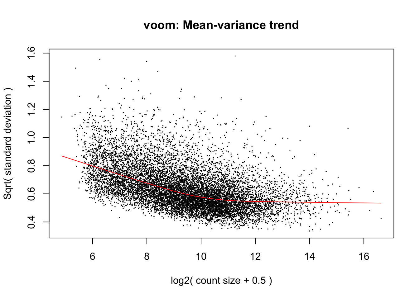
fit <- lmFit(cpm.voom.corfit , design, block=individual, correlation=corfit.correlation)


# Effect size

effect_size <- as.data.frame(fit)

# Log2(CPM) C day 0 - log2(CPM) H day 0

div_day0 <- effect_size[,1] - effect_size[,5]

# Log2(CPM) C day 1 - log2(CPM) H day 1

div_day1 <- effect_size[,2] - effect_size[,6]


# Make a dataframe with all
divergence_01 <- cbind(div_day0, div_day1)

colnames(divergence_01) <- c("0", "1")

boxplot(divergence_01, ylab = "Effect size (chimpanzee - human)", main = "Divergence at days 0-1", xlab = "Day")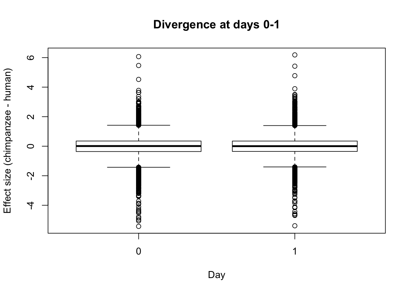
# Perform t tests to look at differences in distributions of effect sizes
t.test(div_day0, div_day1)
    Welch Two Sample t-test

data:  div_day0 and div_day1
t = -0.57184, df = 20578, p-value = 0.5674
alternative hypothesis: true difference in means is not equal to 0
95 percent confidence interval:
 -0.02431531  0.01333198
sample estimates:
  mean of x   mean of y
-0.01931267 -0.01382100
# t = -0.62268, df = 20576, p-value = 0.5335
# Make the dataframe for ggplot2
day0_array <- array("0", dim = c(10304,1))
day1_array <- array("1", dim = c(10304,1))
divergence_day0 <- cbind(as.data.frame((div_day0)), as.factor(day0_array))
colnames(divergence_day0) <- c("Effect_size", "Day")
divergence_day1 <- cbind(as.data.frame(div_day1), day1_array)
colnames(divergence_day1) <- c("Effect_size", "Day")
divergence_plot <- rbind(divergence_day0, divergence_day1)
divergence_plot$Effect_size <- as.numeric(divergence_plot[,1])
ggplot(data=divergence_plot, aes(x=as.factor(Day), y=Effect_size)) + geom_boxplot() + xlab("Day") + ylab("Effect size Difference (Chimp - Human)") + theme_bw() + labs(title = "Divergence")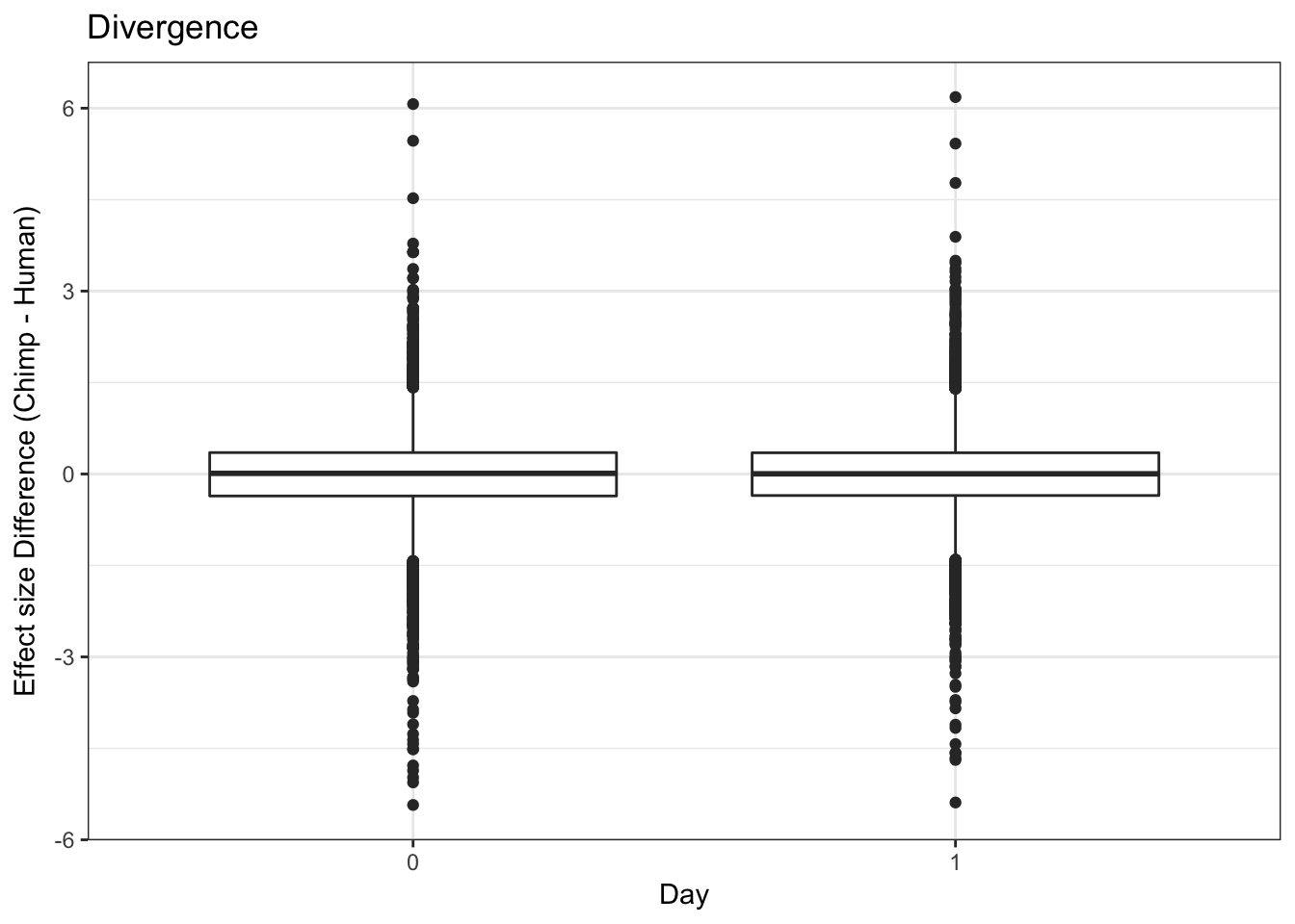
Data visualization (subset of samples, 2-3 humans)
# Make PCA plots with the factors colored by day
#pca_genes <- prcomp(t(cpm_in_cutoff), scale = T, retx = TRUE, center = TRUE)
#scores <- pca_genes$x
#matrixpca <- pca_genes$x
#pc1 <- matrixpca[,1]
#pc2 <- matrixpca[,2]
#pc3 <- matrixpca[,3]
#pc4 <- matrixpca[,4]
#pc5 <- matrixpca[,5]
#pcs <- data.frame(pc1, pc2, pc3, pc4, pc5)
#summary <- summary(pca_genes)
#ggplot(data=pcs, aes(x=pc1, y=pc2, color=as.factor(day1), shape=as.factor(species1), size=2)) + geom_point() + xlab(paste("PC1 (",(summary$importance[2,1]*100), "% of variance)")) + ylab(paste("PC2 (",(summary$importance[2,2]*100), "% of variance)")) + guides(color = guide_legend(order=1), size = FALSE, shape = guide_legend(order=2)) + scale_color_discrete(name ="Day") + labs(title = "PCA of normalized endoderm data (Humans subset to match chimps)")DE genes by species at each time point using only the genes that remained post-filtering for STEM
# Use only the genes from the final step of the STEM analysis
STEM_post_filtering_ensg_only <- read.csv("~/Desktop/Endoderm_TC/ashlar-trial/data/STEM_post_filtering_ensg_only.txt", sep="")
inshared_lists = row.names(genes_in_cutoff) %in% STEM_post_filtering_ensg_only$ensg
inshared_lists_data <- as.data.frame(inshared_lists)
STEM_gene_number <- which(inshared_lists_data=='TRUE')
cpm_in_cutoff_STEM_genes <- cpm(dge_in_cutoff[STEM_gene_number,], normalized.lib.sizes=TRUE, log=TRUE)
cpm.voom_STEM <- voom(dge_in_cutoff[STEM_gene_number,], design, normalize.method="none")
# We want a random effect term for individual
#corfit <- duplicateCorrelation(cpm.voom_STEM, design,block=individual)
corfit.correlation = 0.2024655
cpm.voom.corfit_STEM <- voom(dge_in_cutoff[STEM_gene_number,], design, plot = TRUE, normalize.method="none", block=individual, correlation = corfit.correlation )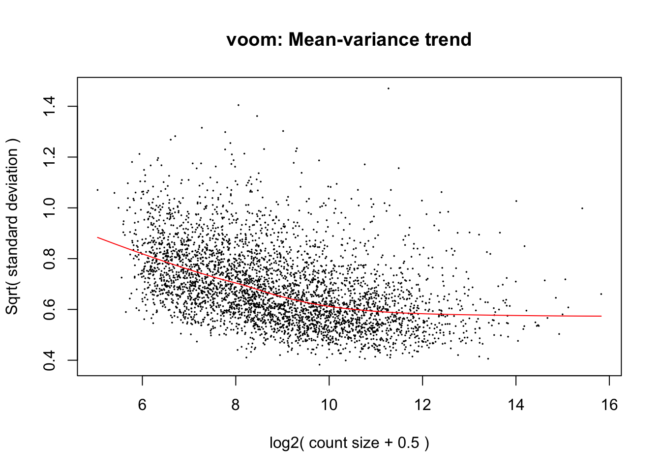
# Run lmFit and eBayes in limma
fit <- lmFit(cpm.voom.corfit_STEM , design, block=individual, correlation=corfit.correlation)
# In the contrast matrix, we have the species DE at each day
cm2 <- makeContrasts(HCday0 = c(1,0,0,0,-1,0,0,0), HCday1 = c(0,1,0,0,0,-1,0,0), HCday2 = c(0,0,1,0,0,0,-1,0), HCday3 = c(0,0,0,1,0,0,0,-1), Hday01 = c(0,0,0,0,1,-1, 0, 0), Hday12 = c(0,0,0,0,0,1,-1,0), Hday23 = c(0,0,0,0,0,0,1,-1), Cday01 = c(1,-1,0,0,0,0,0,0), Cday12 = c(0,1,-1,0,0,0,0,0), Cday23 = c(0,0,1,-1, 0,0,0,0), levels = design)
# Fit the new model
diff_species <- contrasts.fit(fit, cm2)
fit2 <- eBayes(diff_species)
top3 <- list(HvCday0 =topTable(fit2, coef=1, adjust="BH", number=Inf, sort.by="none"), HvCday1 =topTable(fit2, coef=2, adjust="BH", number=Inf, sort.by="none"), HvCday2 =topTable(fit2, coef=3, adjust="BH", number=Inf, sort.by="none"), HvCday3 =topTable(fit2, coef=4, adjust="BH", number=Inf, sort.by="none"), Hday01 =topTable(fit2, coef=5, adjust="BH", number=Inf, sort.by="none"), Hday12 =topTable(fit2, coef=6, adjust="BH", number=Inf, sort.by="none"), Hday23 =topTable(fit2, coef=7, adjust="BH", number=Inf, sort.by="none"), Cday01 =topTable(fit2, coef=8, adjust="BH", number=Inf, sort.by="none"), Cday12 =topTable(fit2, coef=9, adjust="BH", number=Inf, sort.by="none"), Cday23 =topTable(fit2, coef=10, adjust="BH", number=Inf, sort.by="none"))
# Set FDR level at 5%
FDR_level <- 0.05
# Pull out DE across species at each day
mylist <- list()
mylist[["DE Day 0"]] <- row.names(top3[[names(top3)[1]]])[top3[[names(top3)[1]]]$adj.P.Val < FDR_level]
mylist[["DE Day 1"]] <- row.names(top3[[names(top3)[2]]])[top3[[names(top3)[2]]]$adj.P.Val < FDR_level]
mylist[["DE Day 2"]] <- row.names(top3[[names(top3)[3]]])[top3[[names(top3)[3]]]$adj.P.Val < FDR_level]
mylist[["DE Day 3"]] <- row.names(top3[[names(top3)[4]]])[top3[[names(top3)[4]]]$adj.P.Val < FDR_level]
# Make as pdf
Four_comp <- venn.diagram(mylist, filename= NULL, main="DE genes between species per day (5% FDR; 3940 genes with log2 fold change >= 1)", cex=1.5 , fill = pal[1:4], lty=1, height=2000, width=3000)
pdf(file = "DE_by_species_3940_STEM_genes.pdf")
grid.draw(Four_comp)
dev.off()quartz_off_screen
2 mylist_humans_by_day <- list()
mylist_humans_by_day[["DE Days 0 to 1"]] <- row.names(top3[[names(top3)[5]]])[top3[[names(top3)[5]]]$adj.P.Val < FDR_level]
mylist_humans_by_day[["DE Days 1 to 2"]] <- row.names(top3[[names(top3)[6]]])[top3[[names(top3)[6]]]$adj.P.Val < FDR_level]
mylist_humans_by_day[["DE Days 2 to 3"]] <- row.names(top3[[names(top3)[7]]])[top3[[names(top3)[7]]]$adj.P.Val < FDR_level]
Three_comp_humans <- venn.diagram(mylist_humans_by_day, filename= NULL, main="DE genes across days in humans (5% FDR)", cex=1.5 , fill = pal[1:3], lty=1, height=2000, width=3000)
pdf(file = "Humans_day_3940_STEM_genes.pdf")
grid.draw(Three_comp_humans)
dev.off()quartz_off_screen
2 mylist_chimps_by_day <- list()
mylist_chimps_by_day[["DE Days 0 to 1"]] <- row.names(top3[[names(top3)[8]]])[top3[[names(top3)[8]]]$adj.P.Val < FDR_level]
mylist_chimps_by_day[["DE Days 1 to 2"]] <- row.names(top3[[names(top3)[9]]])[top3[[names(top3)[9]]]$adj.P.Val < FDR_level]
mylist_chimps_by_day[["DE Days 2 to 3"]] <- row.names(top3[[names(top3)[10]]])[top3[[names(top3)[10]]]$adj.P.Val < FDR_level]
Three_comp_chimps <- venn.diagram(mylist_chimps_by_day, filename= NULL, main="DE genes across days in chimpanzees (5% FDR)", cex=1.5 , fill = pal[1:3], lty=1, height=2000, width=3000)
pdf(file = "Chimps_day_3940_STEM_genes.pdf")
grid.draw(Three_comp_chimps)
dev.off()quartz_off_screen
2