PART ONE: See if any of the variables for RNA-Seq correlate with the expression PCs for genes (63 samples)
PART TWO: For the variable(s) that correlate, see if these segregate with either species or tissue
PART THREE: Which variables to consider putting in the model?
PART FOUR: See if any of the variables for RNA-Seq correlate with the expression PCs for genes (40 samples)

The goal of this is to establish which, if any, technical factors are correlated with our biological variables of interest.

PART ONE: See if any of the variables for RNA-Seq correlate with the expression PCs for genes (63 samples)

Initialization

# Load libraries

library("gdata")

## gdata: read.xls support for 'XLS' (Excel 97-2004) files ENABLED.

##

## gdata: read.xls support for 'XLSX' (Excel 2007+) files ENABLED.

## 
## Attaching package: 'gdata'

## The following object is masked from 'package:stats':
## 
##     nobs

## The following object is masked from 'package:utils':
## 
##     object.size

library("ggplot2")

## Warning: package 'ggplot2' was built under R version 3.2.5

## Warning in FUN(X[[i]], ...): failed to assign NativeSymbolInfo for env
## since env is already defined in the 'lazyeval' namespace

library("qvalue")

## Warning: package 'qvalue' was built under R version 3.2.3

library("glmnet")

## Warning: package 'glmnet' was built under R version 3.2.5

## Loading required package: Matrix

## Warning: package 'Matrix' was built under R version 3.2.5

## Loading required package: foreach

## Loaded glmnet 2.0-10

source("~/Desktop/Endoderm_TC/ashlar-trial/analysis/chunk-options.R")

## Warning: package 'knitr' was built under R version 3.2.5

# Load cpm data 

cpm_in_cutoff <- read.delim("../data/cpm_cyclicloess.txt")

# Load sample information

After_removal_sample_info <- read.csv("~/Desktop/Endoderm_TC/After_removal_sample_info.csv")

Species <- After_removal_sample_info$Species
species <- After_removal_sample_info$Species
day <- After_removal_sample_info$Day
individual <- After_removal_sample_info$Individual
Sample_ID <- After_removal_sample_info$Sample_ID
labels <- paste(Sample_ID, day, sep=" ")

# Load technical factor information

RNA_seq_info_all <- read.csv("../data/Endo_TC_Data_Share_Sorting.csv",  header = T)

dim(RNA_seq_info_all)

## [1] 130  43

RNA_seq_info <- as.data.frame(cbind(RNA_seq_info_all[1:63, 4], RNA_seq_info_all[1:63, 3], RNA_seq_info_all[1:63, 5:27], RNA_seq_info_all[1:63, 30:35], RNA_seq_info_all[1:63, 37:43]))

# Remove library well (only 1/well)
RNA_seq_info <- RNA_seq_info[,-20]

# Full data set
dim(RNA_seq_info)

## [1] 63 37

Obtain gene expression PCs

# PCs

pca_genes <- prcomp(t(cpm_in_cutoff), scale = T, retx = TRUE, center = TRUE)

matrixpca <- pca_genes$x
pc1 <- matrixpca[,1]
pc2 <- matrixpca[,2]
pc3 <- matrixpca[,3]
pc4 <- matrixpca[,4]
pc5 <- matrixpca[,5]

pcs <- data.frame(pc1, pc2, pc3, pc4, pc5)

summary <- summary(pca_genes)

Plots for PCs versus technical factors

#Create plots for each of the possible confounders versus PCs 1-5

pdf('../data/VarVsGenePCs.pdf')

for (i in 2:length(RNA_seq_info)) { 
  par(mfrow=c(1,5))
  plot(RNA_seq_info[,i], pcs[,1],  ylab = "PC1", xlab = " ")
  plot(RNA_seq_info[,i], pcs[,2],  ylab = "PC2", xlab = " ")
  plot(RNA_seq_info[,i], pcs[,3],  ylab = "PC3", xlab = " ")
  plot(RNA_seq_info[,i], pcs[,4],  ylab = "PC4", xlab = " ")
  plot(RNA_seq_info[,i], pcs[,5],  ylab = "PC5", xlab = " ")
  title(xlab = substitute(paste(k), list(k=colnames(RNA_seq_info)[i])), outer = TRUE, line = -2)
  mtext(substitute(paste('PCs vs. ', k), list(k=colnames(RNA_seq_info)[i])), side = 3, line = -2, outer = TRUE)

}
dev.off()

quartz_off_screen 
                2

Testing association between a particular variable and PCs with a linear model

# TESTING BIOLOGICAL VARIABLES OF INTEREST

PC_pvalues_day = matrix(data = NA, nrow = 5, ncol = 1, dimnames = list(c("PC1", "PC2", "PC3", "PC4", "PC5"), c("Day")))

for(i in 1:5){
# PC versus day

 checkPC1 <- lm(pcs[,i] ~ as.factor(day))

#Get the summary statistics from it
  summary(checkPC1)

#Get the p-value of the F-statistic
  summary(checkPC1)$fstatistic

  fstat <- as.data.frame(summary(checkPC1)$fstatistic)
  p_fstat <- 1-pf(fstat[1,], fstat[2,], fstat[3,])
  PC_pvalues_day[i,1] <- p_fstat
  
#Fraction of the variance explained by the model
  r2_value <- summary(checkPC1)$r.squared

}
# PC  versus species

PC_pvalues_species = matrix(data = NA, nrow = 5, ncol = 1, dimnames = list(c("PC1", "PC2", "PC3", "PC4", "PC5"), c("Species")))

for(i in 1:5){
# PC versus species

   checkPC1 <- lm(pcs[,i] ~ as.factor(species))

#Get the summary statistics from it
  summary(checkPC1)

#Get the p-value of the F-statistic
  summary(checkPC1)$fstatistic

  fstat <- as.data.frame(summary(checkPC1)$fstatistic)
  p_fstat <- 1-pf(fstat[1,], fstat[2,], fstat[3,])
  PC_pvalues_species [i,1] <- p_fstat 
  
#Fraction of the variance explained by the model
  r2_value <- summary(checkPC1)$r.squared
}

# TESTING TECHNICAL VARIABLES OF INTEREST
  
#Make an empty matrix to put all of the data in
# Note: Do not include TC day, as it is a biological variable of interest

PC_pvalues = matrix(data = NA, nrow = 5, ncol = 35, dimnames = list(c("PC1", "PC2", "PC3", "PC4", "PC5"), c("Cell line",  "Batch", "Sex", "Passage at seed",  "Start date", "Density at seed", "Harvest time", "Harvest density", "Purity", "Max purity", "RNA Extraction Date", "RNA conc", "RIN", "260 280 RNA", "260 230 RNA", "DNA concentration", "Library prep batch", "Library concentration", "uL sample", "uL EB", "Index sequence", "Seq pool", "Lane r1", "Mseqs R1", "Total lane reads 1", "Lane prop r1", "Dup r1", "GC r1", "Lane r2", "Mseqs r2", "Total lane reads r2", "Lane prop r2", "Dups r2", "GC r2", "Total reads")))

PC_r2 = matrix(data = NA, nrow = 5, ncol = 35, dimnames = list(c("PC1", "PC2", "PC3", "PC4", "PC5"), c("Cell line",  "Batch", "Sex", "Passage at seed",  "Start date", "Density at seed",   "Harvest time", "Harvest density", "Purity", "Max purity", "RNA Extraction Date", "RNA conc", "RIN", "260 280 RNA", "260 230 RNA", "DNA concentration", "Library prep batch", "Library concentration", "uL sample", "uL EB", "Index sequence", "Seq pool", "Lane r1", "Mseqs R1", "Total lane reads 1", "Lane prop r1", "Dup r1", "GC r1", "Lane r2", "Mseqs r2", "Total lane reads r2", "Lane prop r2", "Dups r2", "GC r2", "Total reads")))

# Take out day and species (factors of interest)
RNA_seq_info_35 <- RNA_seq_info[,-(1:2)]

numerical_tech_factors <- c(4, 6,8:10, 12:16,18:20,24:28,30:35)
categorical_tech_factors <- c(1:3, 5,7,11,17,21:23,29)

#Check lm to see how well the variables containing numerical data are correlated with a PC

#For PCs 1-5
j=1
for (i in numerical_tech_factors){
  for (j in 1:5){
  
  checkPC1 <- lm(pcs[,j] ~ RNA_seq_info_35[,i])

#Get the summary statistics from it
  summary(checkPC1)

#Get the p-value of the F-statistic
  summary(checkPC1)$fstatistic

  fstat <- as.data.frame(summary(checkPC1)$fstatistic)
  p_fstat <- 1-pf(fstat[1,], fstat[2,], fstat[3,])
  
#Fraction of the variance explained by the model
  r2_value <- summary(checkPC1)$r.squared

#Put the summary statistics into the matrix w

  PC_pvalues[j, i] <- p_fstat
  PC_r2[j, i] <- r2_value
  
  }

}
#Check lm to see how well the variables containing ordinal data are correlated with a PC

#For PCs 1-5
j=1
for (i in categorical_tech_factors){
  for (j in 1:5){
  
  checkPC1 <- lm(pcs[,j] ~ as.factor(RNA_seq_info_35[,i]))

#Get the summary statistics from it
  summary(checkPC1)

#Get the p-value of the F-statistic
  summary(checkPC1)$fstatistic

  fstat <- as.data.frame(summary(checkPC1)$fstatistic)
  p_fstat <- 1-pf(fstat[1,], fstat[2,], fstat[3,])
  
#Fraction of the variance explained by the model
  r2_value <- summary(checkPC1)$r.squared

#Put the summary statistics into the matrix w

  PC_pvalues[j, i] <- p_fstat
  PC_r2[j, i] <- r2_value
  
  }

}

#write.table(PC_pvalues, "/Users/laurenblake/Desktop/pc_pvalues.txt")

Test for potential violations of the assumptions of the linear model

Note: I learned in http://lauren-blake.github.io/Reg_Evo_Primates/analysis/Tech_factor_analysis1_gene_exp.html that this doesn’t work when one or more cells in a column contains an “NA”.

Find which factors are statistically significant

#Distribution of p-values adjusted by FDR not including species or tissue

fdr_val = p.adjust(PC_pvalues, method = "fdr", n = length(PC_pvalues))
fdr_val_order = fdr_val[order(fdr_val)]
hist(fdr_val_order, ylab = "BH-adjusted p-values", main = "Distribution of Benjamini and Hochberg adjusted p-values", breaks = 10)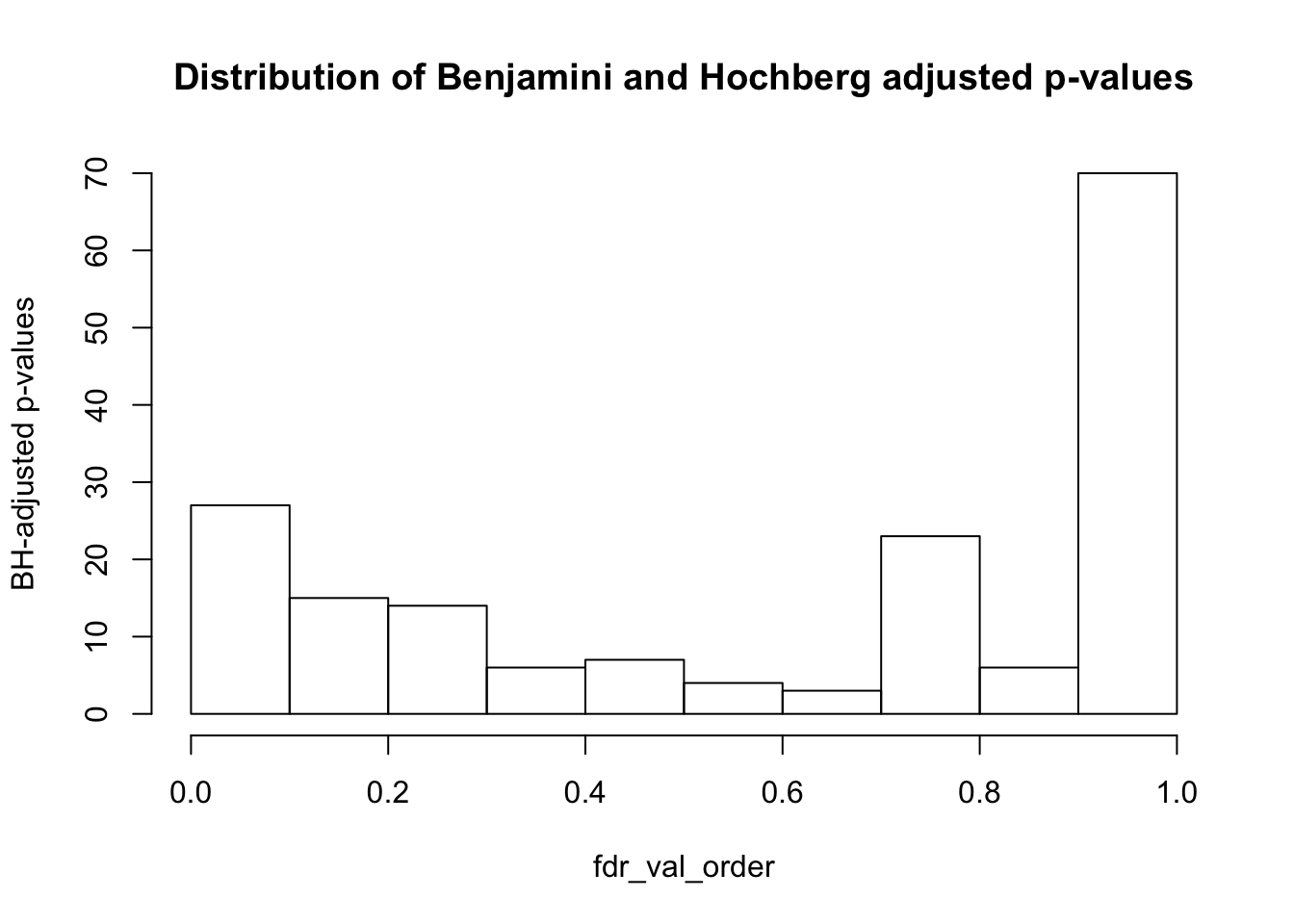

# Number of values significant at 10% FDR 

fdr_val <- matrix(fdr_val, nrow = 5, ncol = 35)
matrix_fdr_val = matrix(data = fdr_val, nrow = 5, ncol = 35, dimnames = list(c("PC1", "PC2", "PC3", "PC4", "PC5"),  c("Cell line",  "Batch", "Sex",  "Passage at seed",  "Start date", "Density at seed", "Harvest time", "Harvest density", "High conf purity", "Max purity", "RNA Extraction Date", "RNA conc", "RIN", "260 280 RNA", "260 230 RNA", "DNA concentration", "Library prep batch", "Library concentration", "uL sample", "uL EB", "Index sequence", "Seq pool", "Lane r1", "Mseqs R1", "Total lane reads 1", "Lane prop r1", "Dup r1", "GC r1", "Lane r2", "Mseqs r2", "Total lane reads r2", "Lane prop r2", "Dups r2", "GC r2", "Total reads")))

#write.table(matrix_fdr_val, "/Users/laurenblake/Desktop/pc_pvalues.txt")

# Number of values significant at 10% FDR 
sum(matrix_fdr_val <= 0.1)

[1] 27

#Get the coordinates of which variables/PC combinations are significant at FDR 10%

TorF_matrix_fdr <- matrix_fdr_val <=0.1
coor_to_check <- which(matrix_fdr_val <= 0.1, arr.ind=T)
coor_to_check <- as.data.frame(coor_to_check)

# Number of variables significant at 10% FDR  (note: off by 1 from column number in RNA_seq_info file; see notes in Part Two)

coor_to_check_col <- coor_to_check$col
unique(coor_to_check_col)

 [1]  1  2  4  5  7  8  9 10 11 12 13 14 17 21 22 23 25 29

** Conclusions from Part I**

The following variables are associated with one of the PCs tested and will be investigated further in Part 2.

Cell line
Batch
Passage at seed
Start date
Harvest time
Harvest density
Purity
Max purity
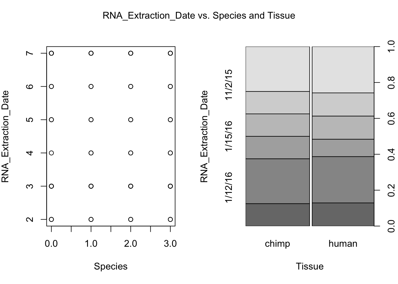
RNA Extraction Date
RNA conc
RIN
260 280 RNA
Library prep batch
Index sequence
Seq pool
Lane r1
Total lane reads 1
Lane r2

PART TWO: For the variable(s) that correlate, see if these segregate with either species or tissue

In coor_to_check_col, row is the PC # and col is the column # -1 that is associated with the PC. Want to take the coor_to_check_col column # and add one.

var_numb = unique(coor_to_check_col) 
var.numb <- as.data.frame(var_numb)


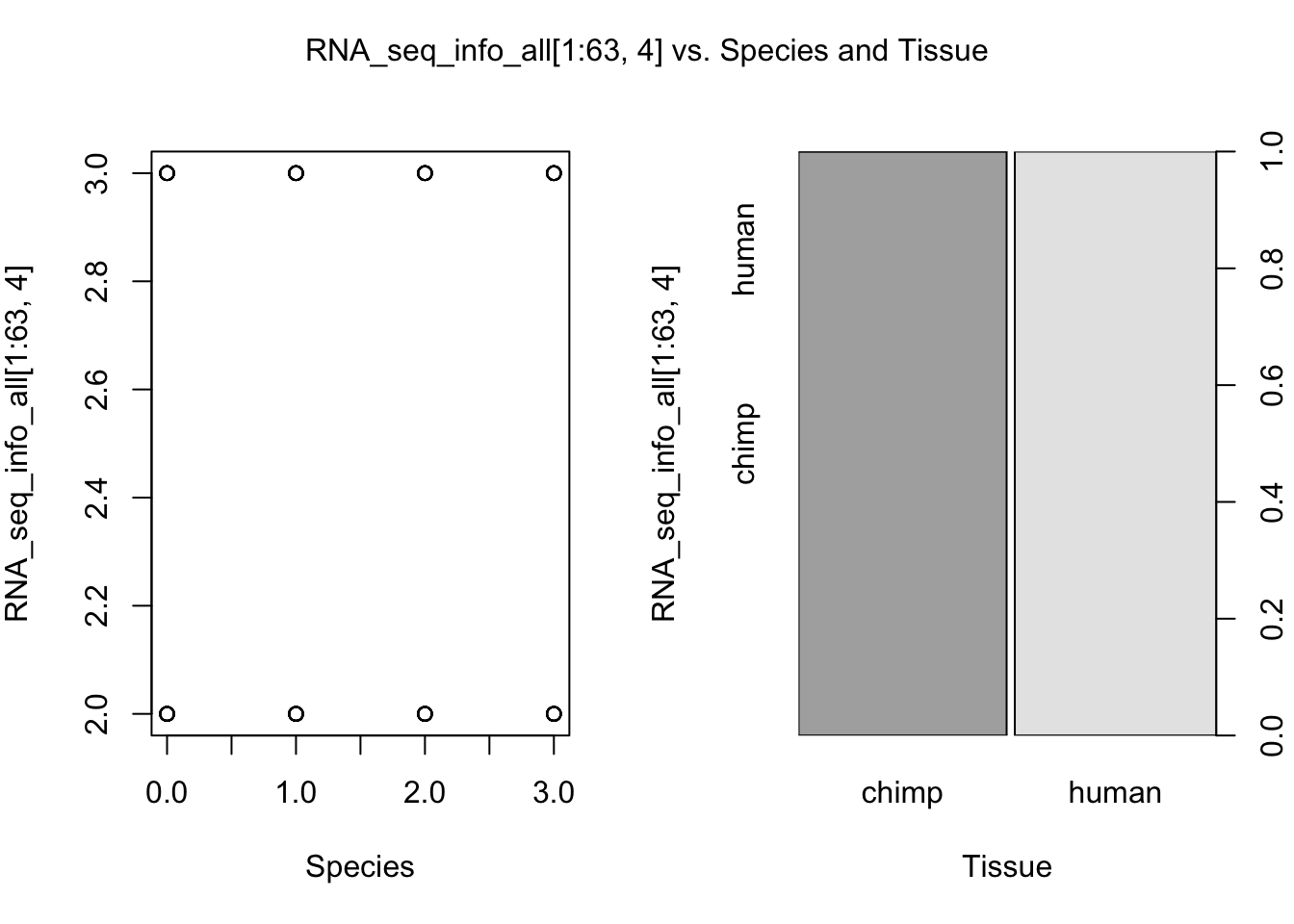
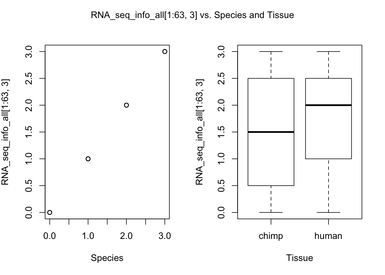
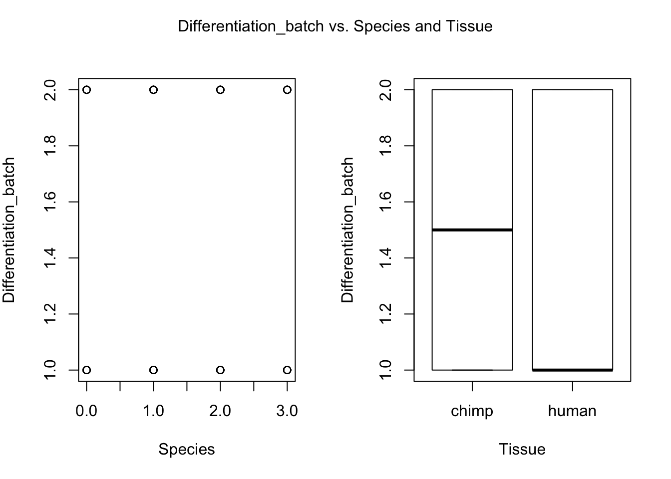
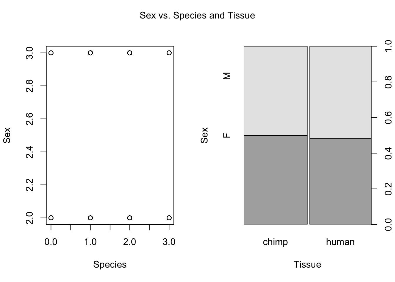
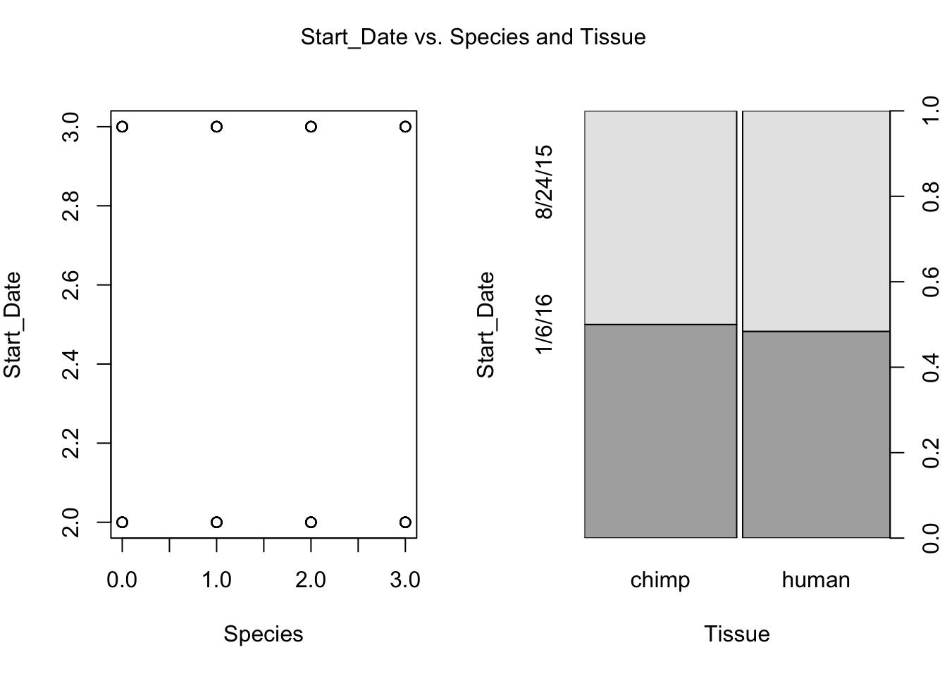
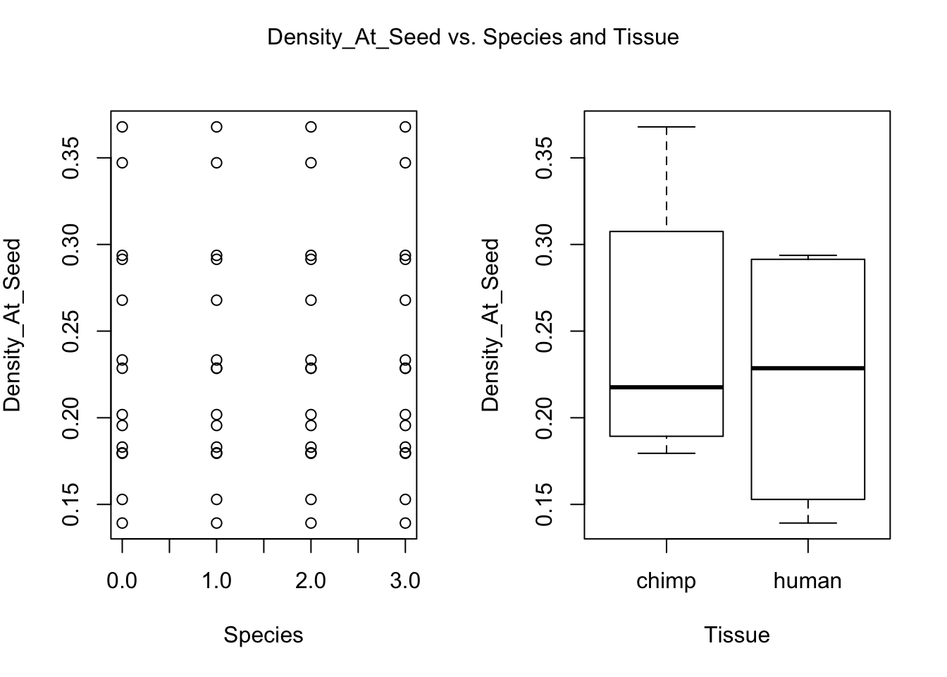
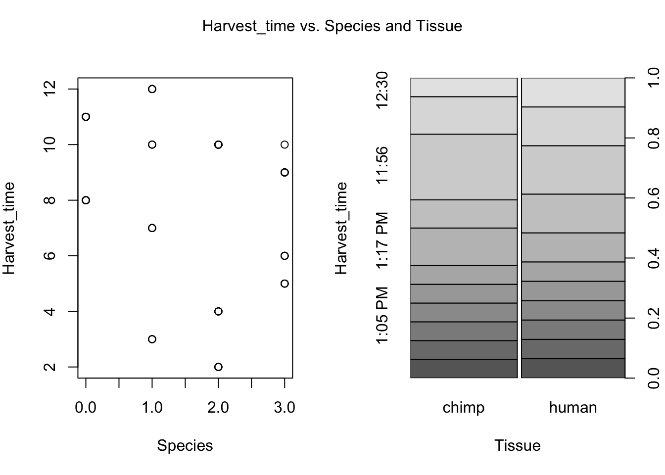
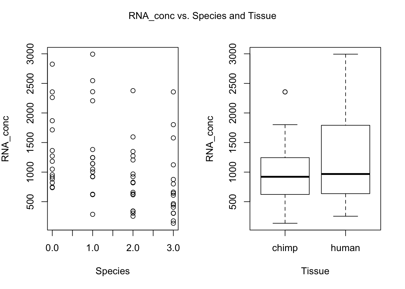
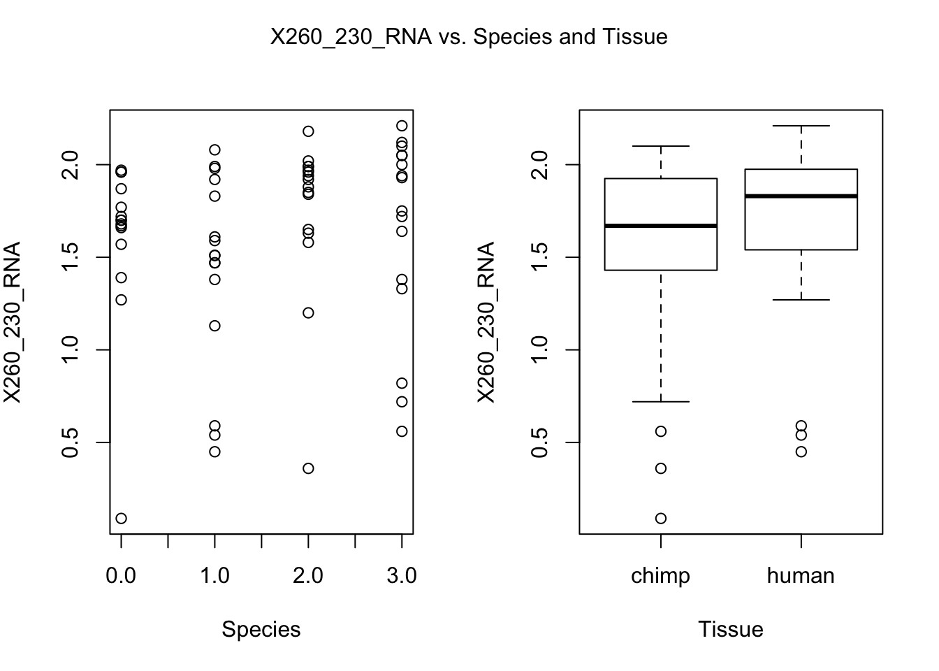
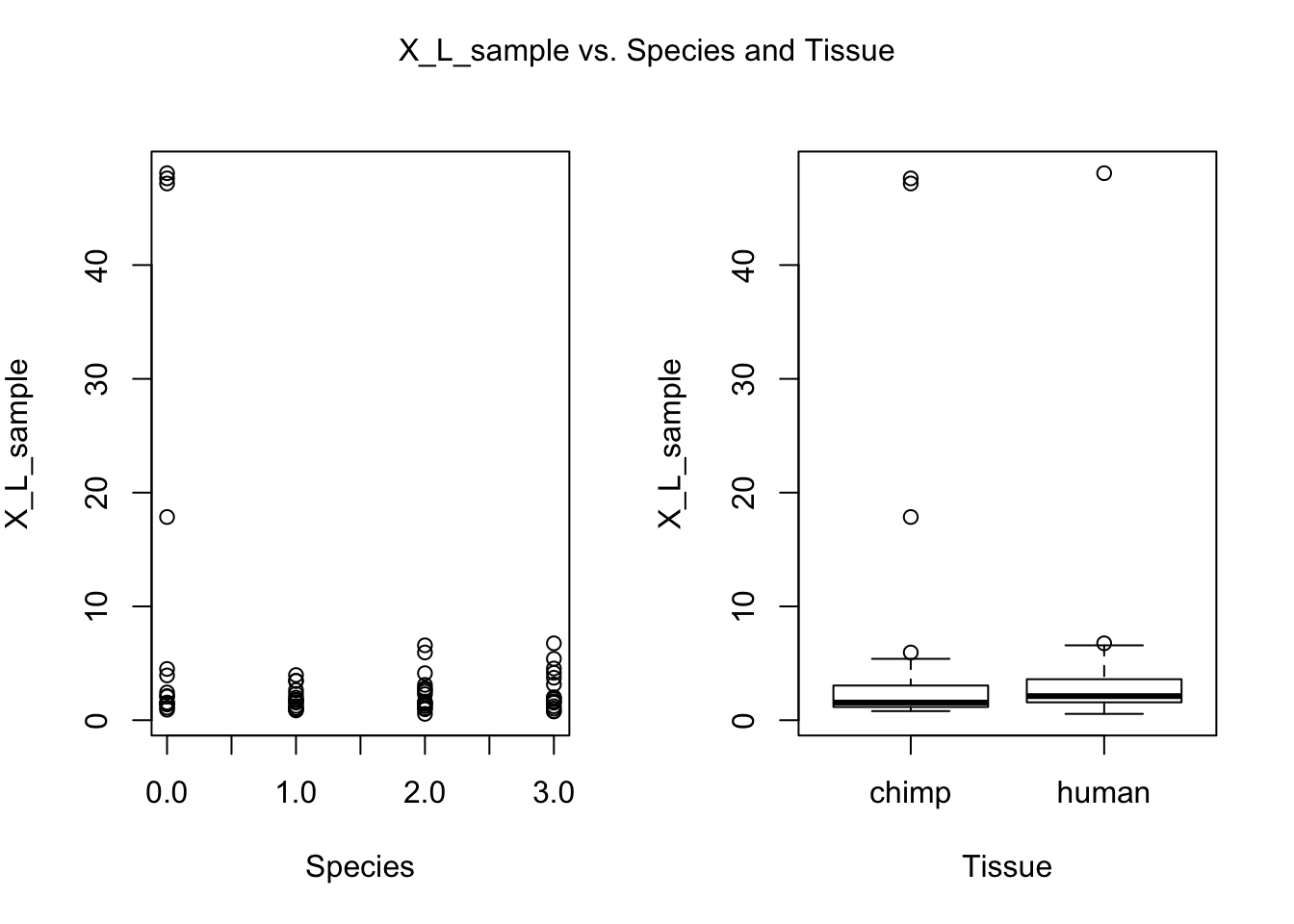
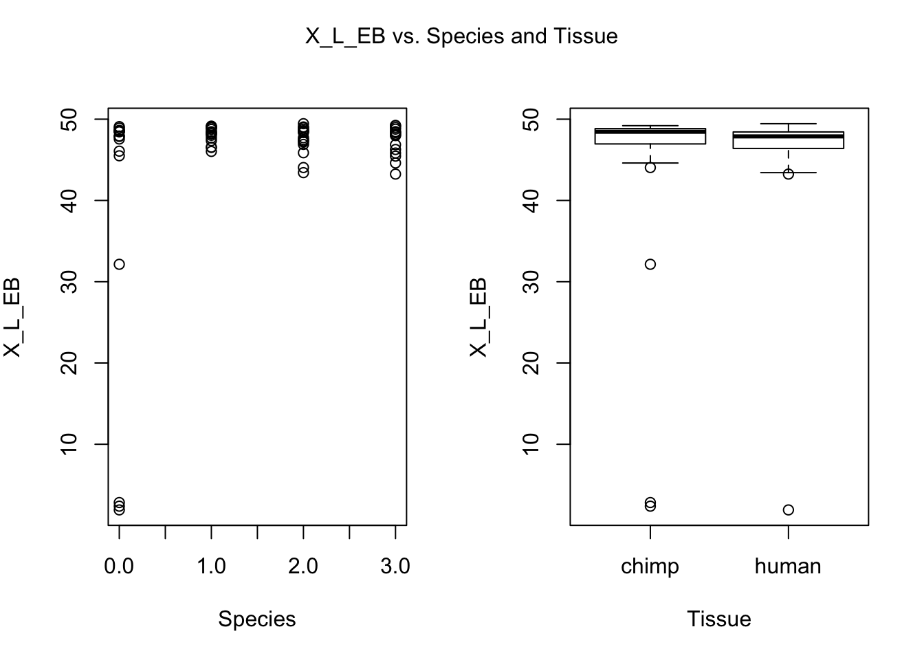
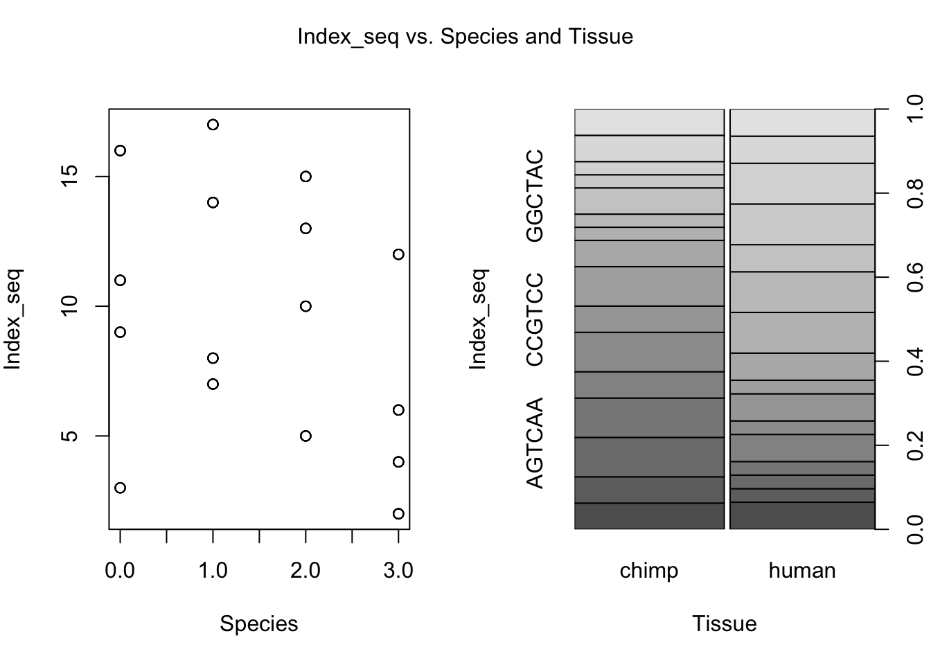
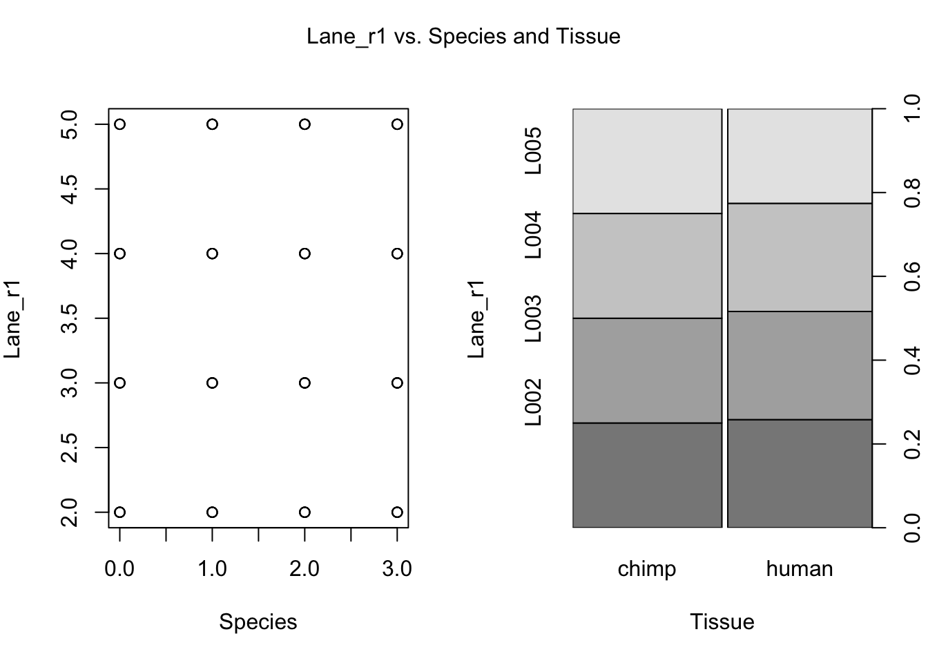
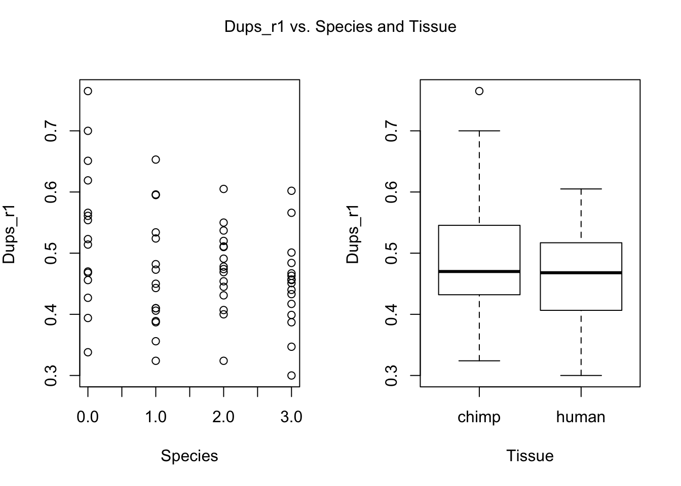
for (i in var.numb[1:nrow(var.numb),]) { 
par(mfrow=c(1,2))
plot(day, RNA_seq_info[,i], xlab = "Species", ylab = substitute(paste(k), list(k=colnames(RNA_seq_info)[i])))

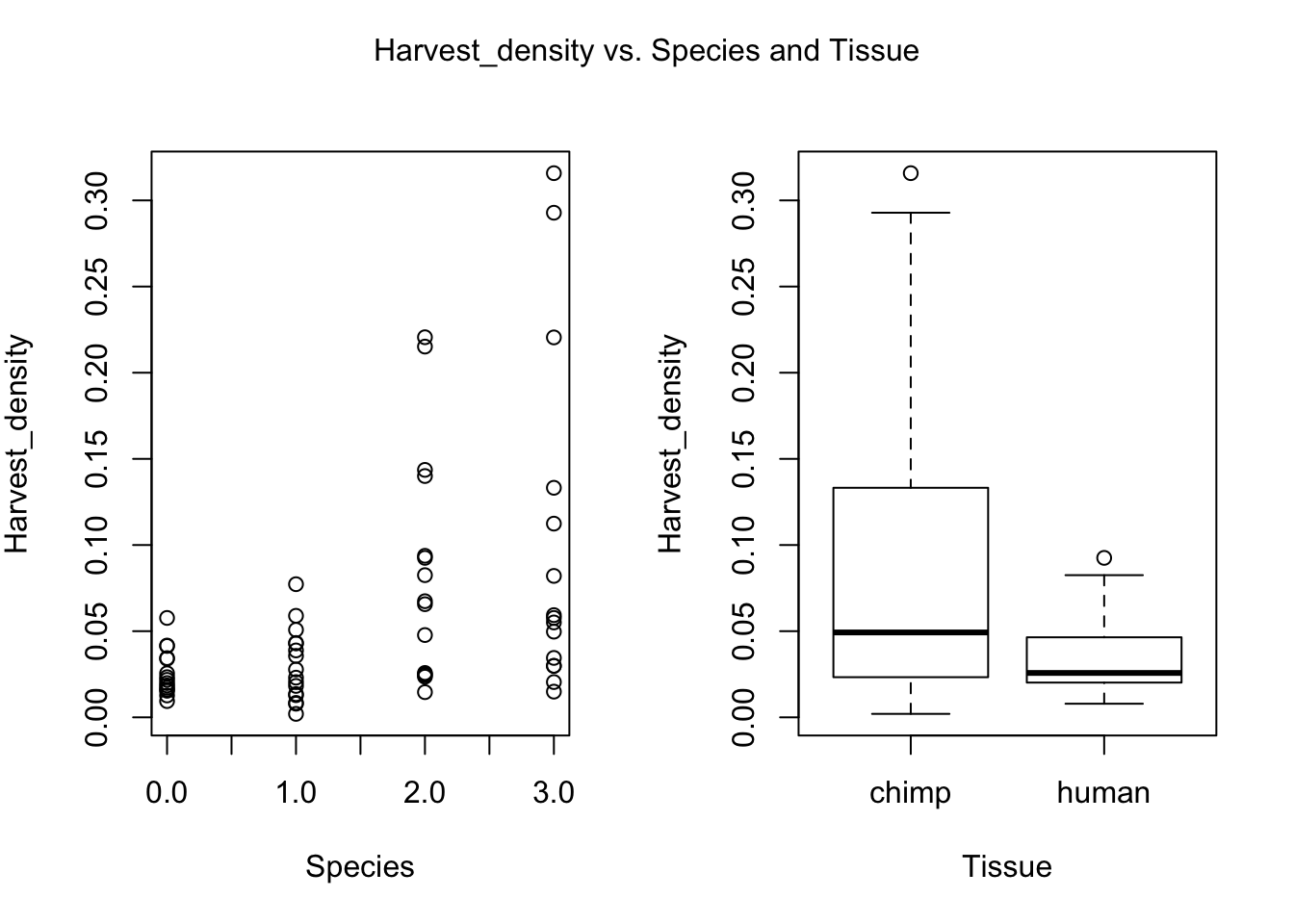
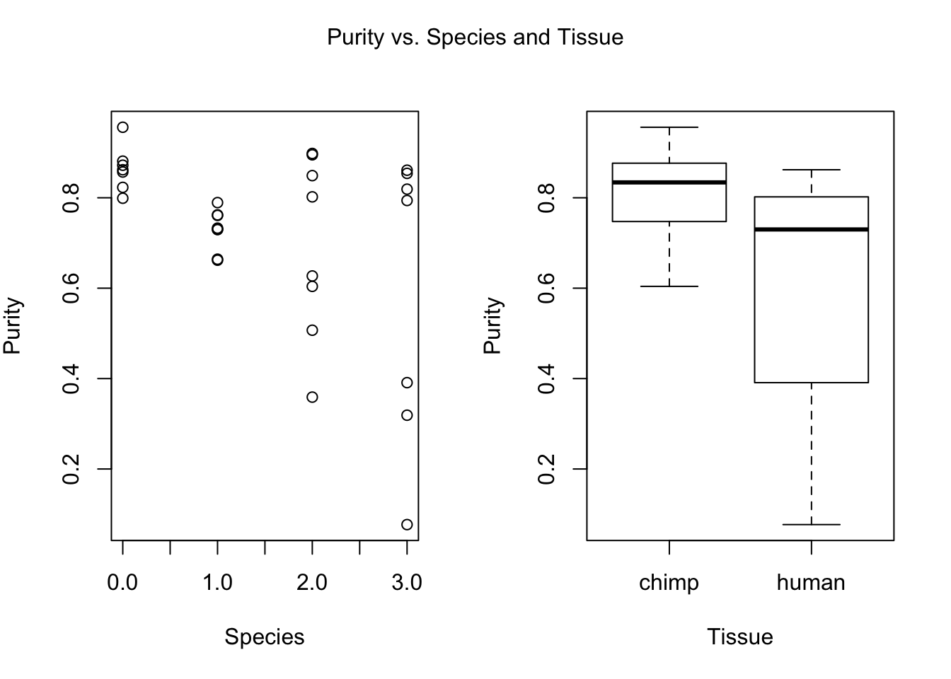
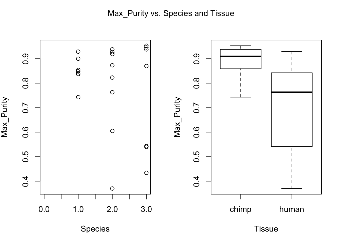
plot(Species, RNA_seq_info[,i], xlab = "Tissue", ylab = substitute(paste(k), list(k=colnames(RNA_seq_info)[i])))

mtext(substitute(paste(k, ' vs. Species and Tissue'), list(k=colnames(RNA_seq_info)[i])), side = 3, line = -2, outer = TRUE)

}

dev.off()

null device 
          1

Testing to see if differences across variable groups are statistically significant for day.

# Technical factors to be tested 

numerical_prev_sign_tech_factors <- c(4, 8:10, 12:14,25) 
categorical_prev_sign_tech_factors <- c(1,2,5,7,11, 17,21:23,29)

#Make a matrix to store the p-values

pvalues_day = matrix(data = NA, nrow = 1, ncol = 35, dimnames = list(c("p-value"),  c("Cell line", "SPSX", "Batch", "Passage at seed",  "Start date", "Density at seed", "Harvest time", "Harvest density", "High conf purity", "Max purity", "RNA Extraction Date", "RNA conc", "RIN", "260 280 RNA", "260 230 RNA", "DNA concentration", "Library prep batch", "Library concentration", "uL sample", "uL EB", "Index sequence", "Seq pool", "Lane r1", "Mseqs R1", "Total lane reads 1", "Lane prop r1", "Dup r1", "GC r1", "Lane r2", "Mseqs r2", "Total lane reads r2", "Lane prop r2", "Dups r2", "GC r2", "Total reads")))

# Numerical

#Performing this test of significance for variables that are numerical data (Using an ANOVA)
j=1
for (i in numerical_prev_sign_tech_factors) {  
summary_anova = summary(aov(RNA_seq_info_35[,i]~ as.factor(day)))
data_summary_anova <- as.data.frame(summary_anova[[1]]$`Pr(>F)`)
p_val_anova <- data_summary_anova[1,]
pvalues_day[, i] <- p_val_anova  
j=j+1
}

# Ordinal

#Performing this test of significance for variables that are categorical data (Using Pearson's chi-squared test)
j=1
for (i in categorical_prev_sign_tech_factors) { 
  
  pval_chi <- chisq.test(as.factor(RNA_seq_info_35[,i]), as.factor(day), simulate.p.value = TRUE)$p.value
  pvalues_day[, i] <- pval_chi  
  j=j+1
  
}

Testing to see if differences across variable groups are statistically significant for species.

# Technical factors to be tested 

numerical_prev_sign_tech_factors <- c(4, 8:10, 12:14,25) 
categorical_prev_sign_tech_factors <- c(1,2,5,7,11, 17,21:23,29)

#Make a matrix to store the p-values

pvalues_species = matrix(data = NA, nrow = 1, ncol = 35, dimnames = list(c("p-value"),  c("Cell line", "Batch", "Sex", "Passage at seed",  "Start date", "Density at seed", "Harvest time", "Harvest density", "High conf purity", "Max purity", "RNA Extraction Date", "RNA conc", "RIN", "260 280 RNA", "260 230 RNA", "DNA concentration", "Library prep batch", "Library concentration", "uL sample", "uL EB", "Index sequence", "Seq pool", "Lane r1", "Mseqs R1", "Total lane reads 1", "Lane prop r1", "Dup r1", "GC r1", "Lane r2", "Mseqs r2", "Total lane reads r2", "Lane prop r2", "Dups r2", "GC r2", "Total reads")))

# Numerical

#Performing this test of significance for variables that are numerical data (Using an ANOVA. Note: in this case, the p-value of the ANOVA is the same as the p-value of the beta1 coefficient in lm)
j=1
for (i in numerical_prev_sign_tech_factors) {  
summary_anova = summary(aov(RNA_seq_info_35[,i]~ as.factor(Species)))
data_summary_anova <- as.data.frame(summary_anova[[1]]$`Pr(>F)`)
p_val_anova <- data_summary_anova[1,]
pvalues_species[, i] <- p_val_anova  
j=j+1
}


# Ordinal

#Performing this test of significance for variables that are categorical data (Using Pearson's chi-squared test)
j=1
for (i in categorical_prev_sign_tech_factors) { 
  
  pval_chi <- chisq.test(as.factor(RNA_seq_info_35[,i]), as.factor(Species), simulate.p.value = TRUE)$p.value
  pvalues_species[, i] <- pval_chi  
  j=j+1
  
}

# Combine tables

collapse_table_full <- rbind(pvalues_day, pvalues_species)

# Want only NAs
collapse_table <- collapse_table_full[, colSums(is.na(collapse_table_full)) != nrow(collapse_table_full)]

#write.table(collapse_table, "/Users/laurenblake/Desktop/collapse_table.txt")

# Harvest density and Species
summary(lm(RNA_seq_info$Harvest_density~ as.factor(Species)))


Call:
lm(formula = RNA_seq_info$Harvest_density ~ as.factor(Species))

Residuals:
     Min       1Q   Median       3Q      Max 
-0.08357 -0.03479 -0.01226  0.01979  0.23023 

Coefficients:
                        Estimate Std. Error t value Pr(>|t|)    
(Intercept)              0.08558    0.01154   7.417 5.31e-10 ***
as.factor(Species)human -0.05029    0.01618  -3.107   0.0029 ** 
---
Signif. codes:  0 '***' 0.001 '**' 0.01 '*' 0.05 '.' 0.1 ' ' 1

Residual standard error: 0.06319 on 59 degrees of freedom
  (2 observations deleted due to missingness)
Multiple R-squared:  0.1406,    Adjusted R-squared:  0.1261 
F-statistic: 9.656 on 1 and 59 DF,  p-value: 0.002902

# Harvest density and Day
summary(lm(RNA_seq_info$Harvest_density~ as.factor(day)))


Call:
lm(formula = RNA_seq_info$Harvest_density ~ as.factor(day))

Residuals:
      Min        1Q    Median        3Q       Max 
-0.085633 -0.028096 -0.007411  0.012799  0.215255 

Coefficients:
                Estimate Std. Error t value Pr(>|t|)   
(Intercept)     0.025926   0.015599   1.662  0.10201   
as.factor(day)1 0.004177   0.021713   0.192  0.84812   
as.factor(day)2 0.059567   0.022061   2.700  0.00911 **
as.factor(day)3 0.074624   0.022061   3.383  0.00130 **
---
Signif. codes:  0 '***' 0.001 '**' 0.01 '*' 0.05 '.' 0.1 ' ' 1

Residual standard error: 0.06042 on 57 degrees of freedom
  (2 observations deleted due to missingness)
Multiple R-squared:  0.2412,    Adjusted R-squared:  0.2012 
F-statistic: 6.039 on 3 and 57 DF,  p-value: 0.001208

chisq.test(as.factor(RNA_seq_info$Harvest_density), as.factor(day), simulate.p.value = TRUE)


    Pearson's Chi-squared test with simulated p-value (based on 2000
    replicates)

data:  as.factor(RNA_seq_info$Harvest_density) and as.factor(day)
X-squared = 183, df = NA, p-value = 0.2339

Find factors with FDR < 0.1

#Calculate q-values (FDR = 10%)

fdr_val = p.adjust(collapse_table, method = "fdr", n = length(collapse_table)*2)
fdr_val_order = fdr_val[order(fdr_val)]
hist(fdr_val_order, ylab = "BH-adjusted p-values", main = "Distribution of Benjamini and Hochberg adjusted p-values", breaks = 10)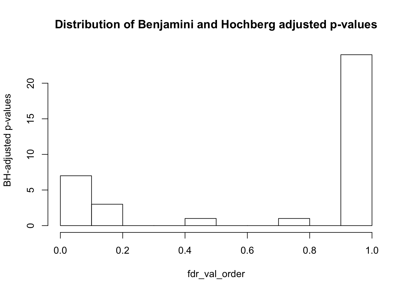

collapse_table_fdr_val = matrix(data = fdr_val, nrow = 2, ncol = nrow(var.numb), dimnames = list(c("Day", "Species"), colnames(collapse_table)))

collapse_table_fdr_val

        Cell line SPSX Passage at seed Start date Harvest time
Day      1.000000    1       1.0000000          1     0.011994
Species  0.011994    1       0.1104767          1     1.000000
        Harvest density High conf purity Max purity RNA Extraction Date
Day          0.02174627       0.48914734 1.00000000                   1
Species      0.03481949       0.08328609 0.03033897                   1
         RNA conc RIN 260 280 RNA Library prep batch Index sequence
Day     0.1580205   1   0.1575861                  1       0.011994
Species 0.7730303   1   1.0000000                  1       1.000000
        Seq pool Lane r1 Total lane reads 1 Lane r2
Day            1       1                  1       1
Species        1       1                  1       1

write.table(collapse_table_fdr_val, "/Users/laurenblake/Desktop/collapse_table_fdr.txt")

** Conclusions from Part 2 **

The following variables are confounded with day:

Harvest time (BH adjusted p-value = 0.011994)
Harvest density (BH adjusted p-value = 0.02174627)
Index sequence (BH adjusted p-value = 0.011994)

The following variables are confounded with species:

Cell line (BH adjusted p-value = 0.011994)
Harvest density (BH adjusted p-value = 0.03481949)
Purity (BH adjusted p-value = 0.08328609)
Max. purity (BH adjusted p-value = 0.03033897)

plot(day, as.factor(RNA_seq_info[,2]), main = "Cell line versus day")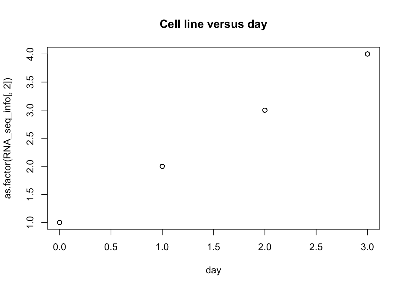

plot(Species, as.factor(RNA_seq_info[,2]), main = "Cell line versus species (sign.)")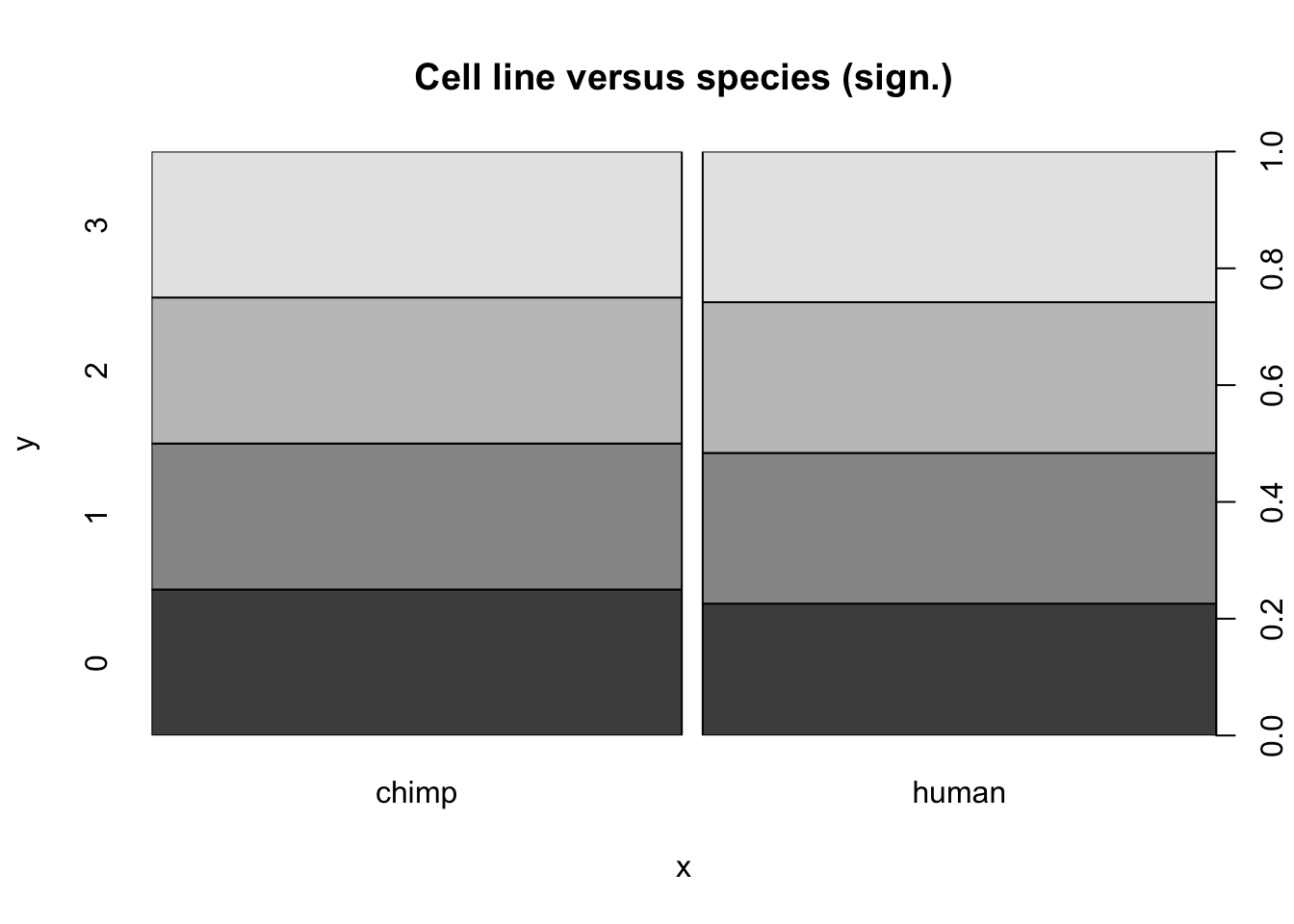

plot(day, as.factor(RNA_seq_info[,3]), main = "SPSX versus day")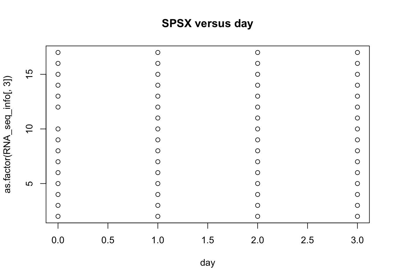

plot(Species, as.factor(RNA_seq_info[,3]), main = "SPSX versus species (sign.)")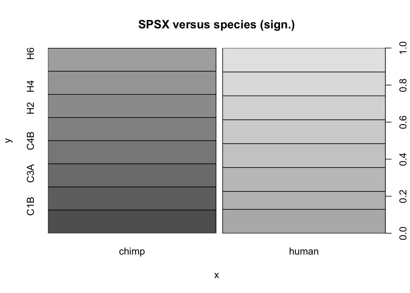

plot(day, as.factor(RNA_seq_info[,8]), main =  "Harvest time versus day (sign.)")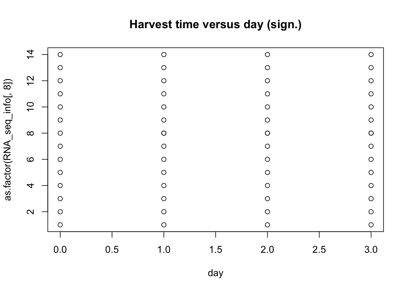

plot(Species, RNA_seq_info[,8], main = "Harvest time versus species")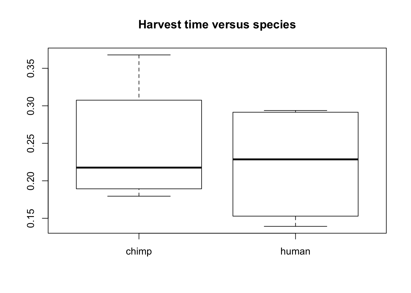

plot(as.factor(day), RNA_seq_info[,9], main = "Harvest density versus day (sign.)", ylab = "Harvest density", xlab = "Day")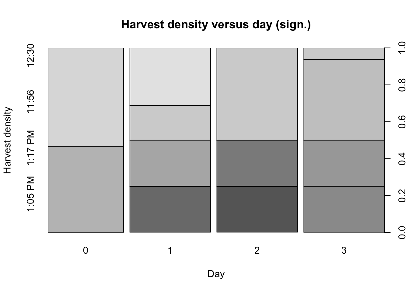

plot(Species, RNA_seq_info[,9], main = "Harvest density versus species (sign.)", ylab = "Harvest density", xlab = "Species")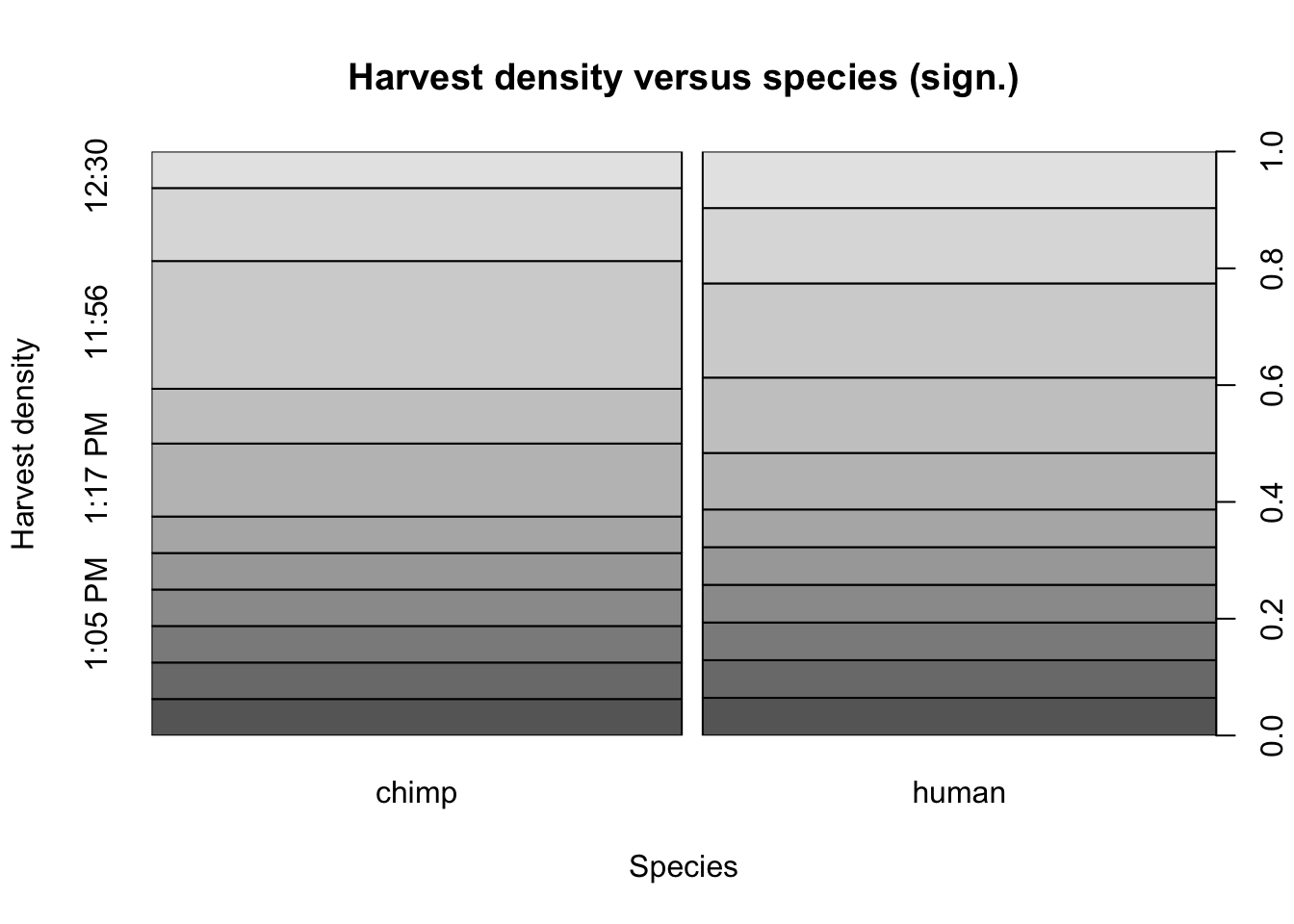

plot(as.factor(day), RNA_seq_info[,10], main = "High confidence purity versus day", ylab = "High confidence purity", xlab = "Day")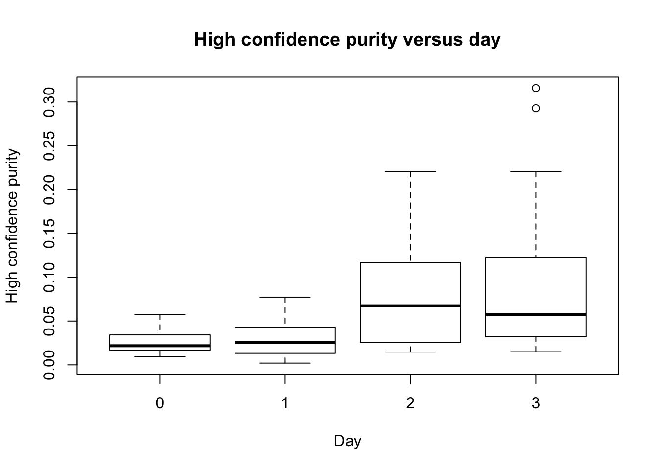

plot(Species, RNA_seq_info[,10], main = "High confidence purity versus species", ylab = "High confidence purity", xlab = "Species")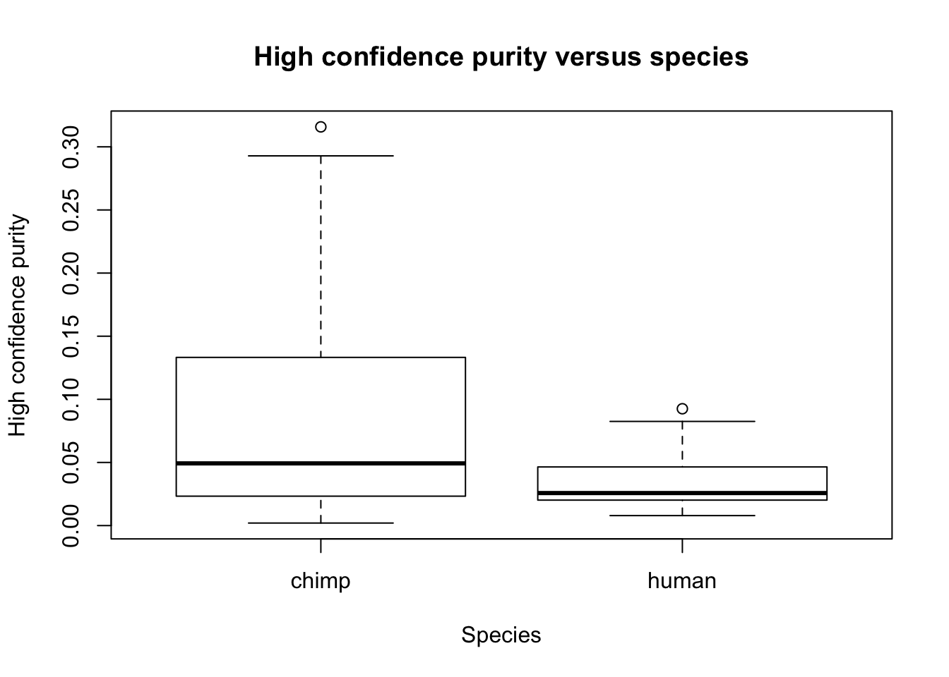

plot(as.factor(day), RNA_seq_info[,11], main = "Max. purity versus day",  ylab = "Max. purity", xlab = "Day")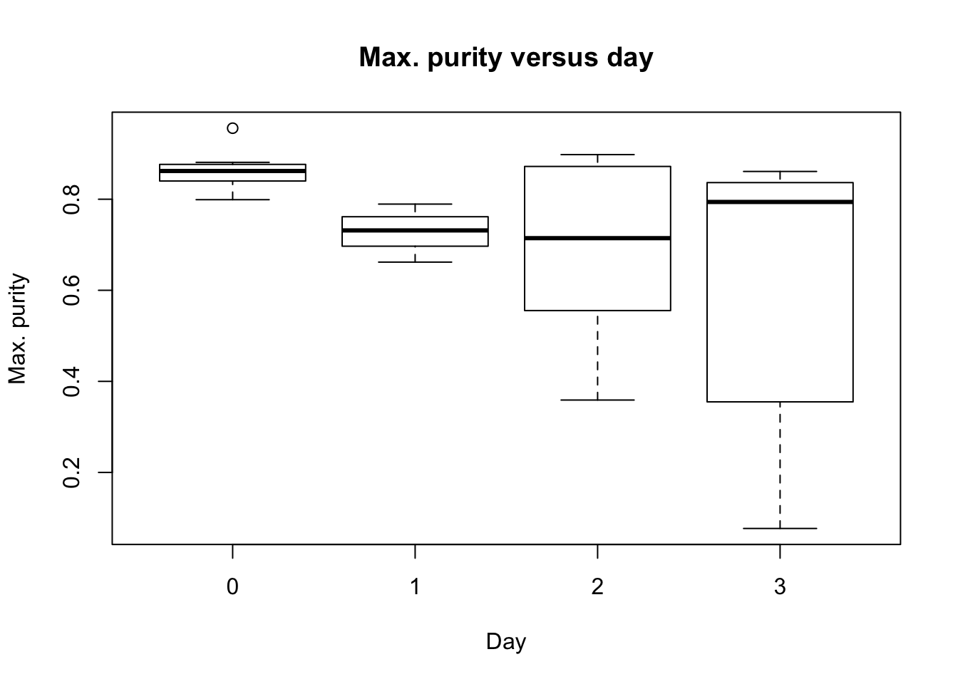

plot(Species, RNA_seq_info[,11], main = "Max. purity versus species (sign.)", ylab = "Max. purity", xlab = "Species")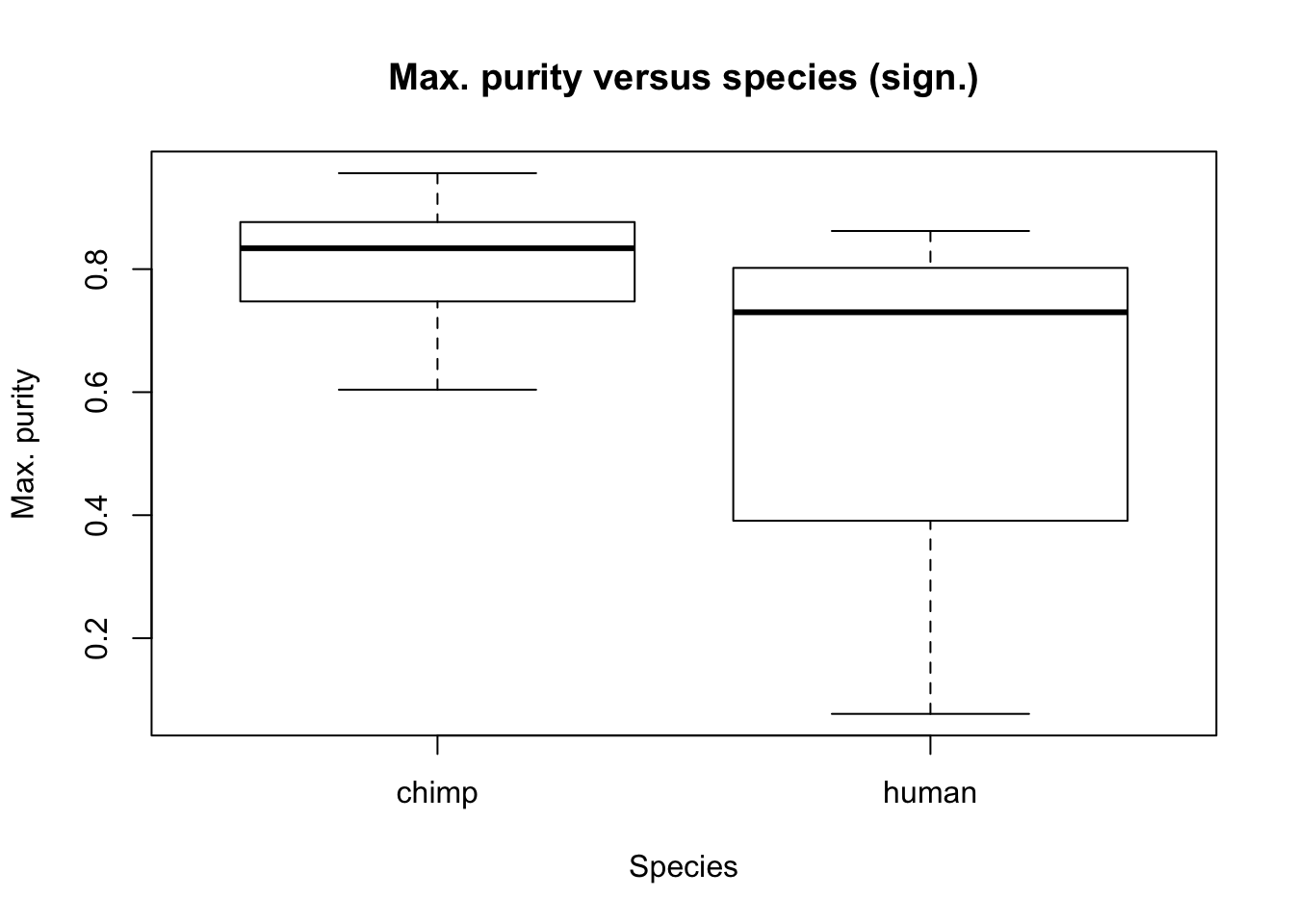

plot(as.factor(day), as.factor(RNA_seq_info[,22]), main = "Index sequence versus day (sign.)")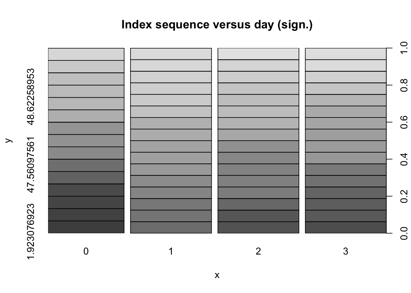

plot(Species, RNA_seq_info[,22], main = "Index sequence versus species")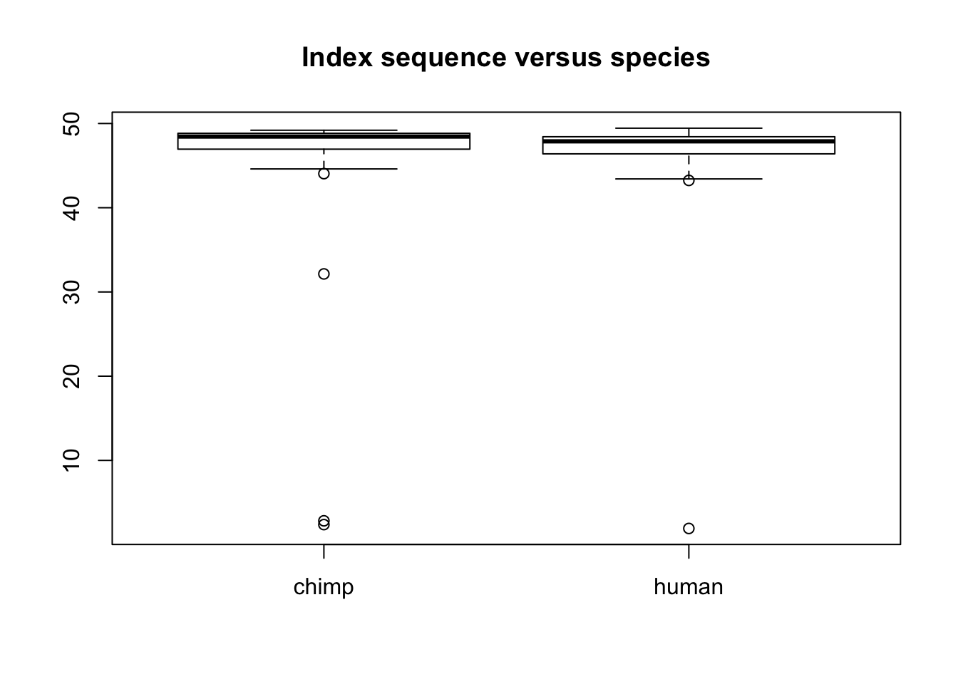

Combine and test day versus adapter for each sequencing pool

# Make table of day, adaptor, and sequencing pool

day_index_pool <- cbind(day, RNA_seq_info$Index_seq, RNA_seq_info$Seq_pool) 

# Test dependency with the adaptors by day 

  # Sequencing pool 1
adaptors_pool1 <- day_index_pool[ which(day_index_pool[,3]==1),]

chisq.test(as.factor(adaptors_pool1[,2]), as.factor(adaptors_pool1[,1]), simulate.p.value = TRUE)$p.value

[1] 1

#fisher.test(adaptors_pool1[,1:2], simulate.p.value=TRUE)$p.value
#fisher.test(adaptors_pool2[,2:1], simulate.p.value=TRUE)$p.value
#fisher.test(adaptors_pool3[,2:1], simulate.p.value=TRUE)$p.value
#fisher.test(adaptors_pool4[,2:1], simulate.p.value=TRUE)$p.value

  # p-value = 1

  # Sequencing pool 2
adaptors_pool2 <- day_index_pool[ which(day_index_pool[,3]==2),]

chisq.test(as.factor(adaptors_pool2[,2]), as.factor(adaptors_pool2[,1]), simulate.p.value = TRUE)$p.value

[1] 1

  # p-value = 1

  # Sequencing pool 3
adaptors_pool3 <- day_index_pool[ which(day_index_pool[,3]==3),]

chisq.test(as.factor(adaptors_pool3[,2]), as.factor(adaptors_pool3[,1]), simulate.p.value = TRUE)$p.value

[1] 1

  # p-value = 1

  # Sequencing pool 4
adaptors_pool4 <- day_index_pool[ which(day_index_pool[,3]==4),]

chisq.test(as.factor(adaptors_pool4[,2]), as.factor(adaptors_pool4[,1]), simulate.p.value = TRUE)$p.value

[1] 1

  # p-value = 1

fdr_val_4= p.adjust(c(1,1,1,1), method = "fdr")
fdr_val_4

[1] 1 1 1 1

PART THREE: Which variables to consider putting in the model?

RIN Score

# Make a table with species, day, and RIN score
species <- After_removal_sample_info$Species
day <- After_removal_sample_info$Day

iPSC_prop <- as.data.frame(cbind(day, species, RNA_seq_info[,14]), stringsAsFactors = FALSE)

# Remove the 1 sample with a missing RIN score

remove_NA <- c(26)

iPSC_prop <- iPSC_prop[-remove_NA, ]

colnames(iPSC_prop) <- c("Day", "Species", "RIN_Score") 

iPSC_prop$Species[iPSC_prop$Species == "2"] <- "Human"
iPSC_prop$Species[iPSC_prop$Species == "1"] <- "Chimp"

iPSC_prop$Day[iPSC_prop$Day == "0"] <- "Day 0"
iPSC_prop$Day[iPSC_prop$Day == "1"] <- "Day 1"
iPSC_prop$Day[iPSC_prop$Day == "2"] <- "Day 2"
iPSC_prop$Day[iPSC_prop$Day == "3"] <- "Day 3"

ggplot(data = iPSC_prop, aes(y = RIN_Score, x = as.factor(Species)))  + facet_wrap(~ Day, nrow = 1) + geom_boxplot() + geom_point(size = 5,  position=position_jitter(width=0.2, height=0.1), show.legend = FALSE) + labs(x = "Species", y = "RIN score") + theme_bw()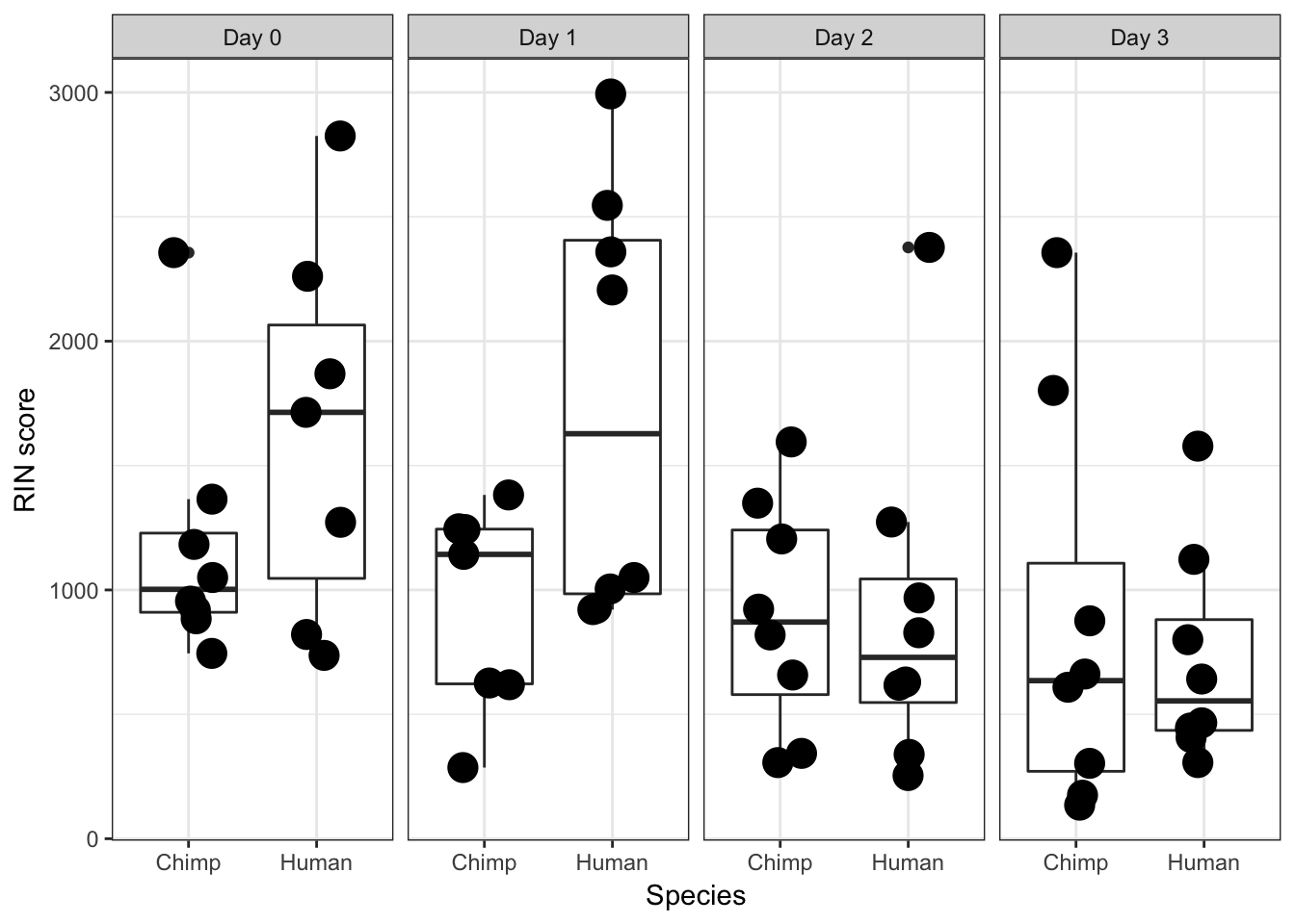

ggplot(data = iPSC_prop, aes(y = RIN_Score, x = as.factor(Species)))  + facet_wrap(~ Day, nrow = 1) + geom_boxplot()  + geom_dotplot(binaxis='y', stackdir='center', binwidth = 0.05) + labs(x = "Species", y = "RIN score") + theme_bw()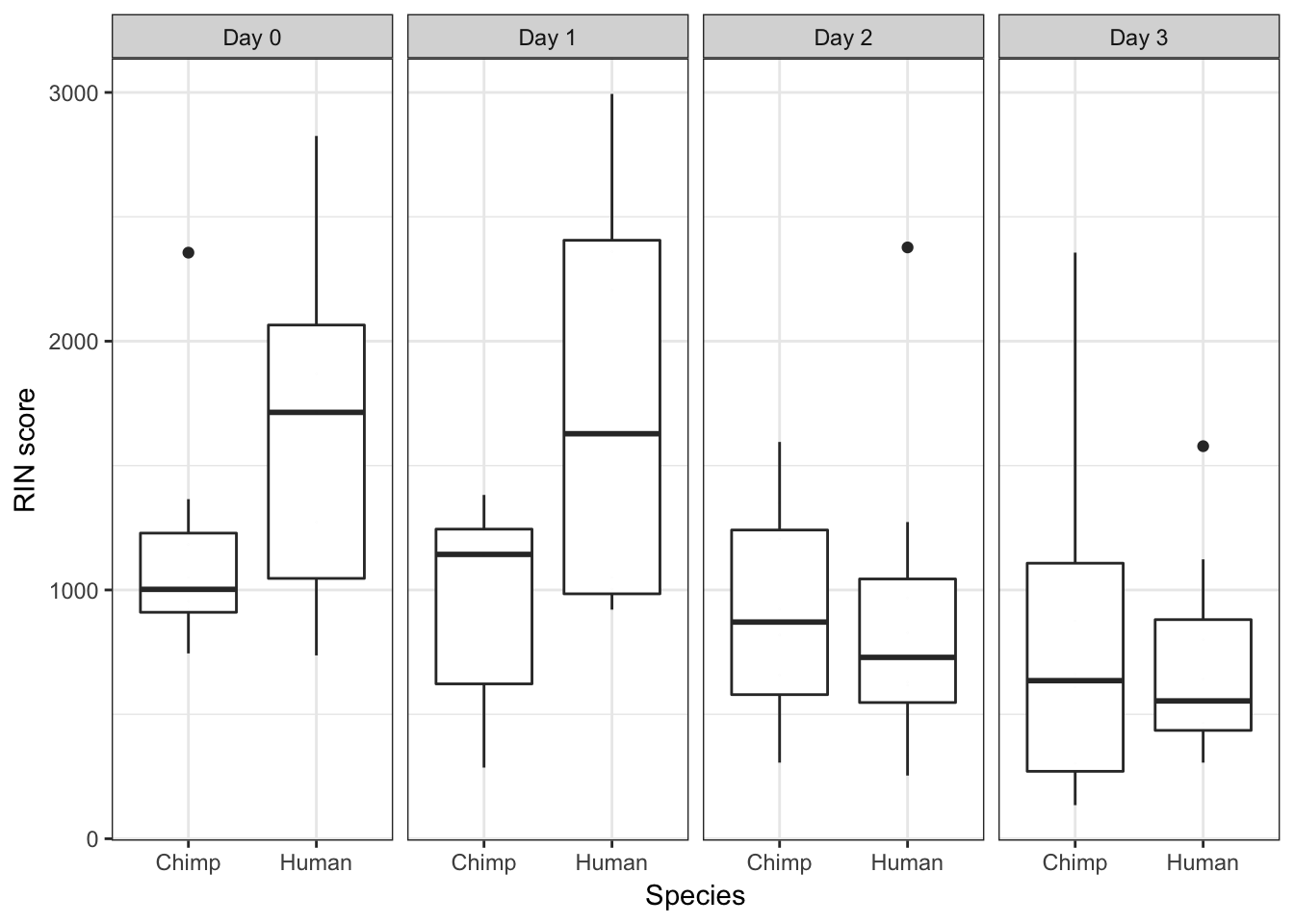

Passage at seed

# Make a table with species, day, and RIN score
species <- After_removal_sample_info$Species
day <- After_removal_sample_info$Day

iPSC_prop <- as.data.frame(cbind(day, species, RNA_seq_info[1:63,35]), stringsAsFactors = FALSE)

# Remove the 1 sample with a missing RIN score

#remove_NA <- c(26)

#iPSC_prop <- iPSC_prop[-remove_NA, ]

colnames(iPSC_prop) <- c("Day", "Species", "RIN_Score") 

iPSC_prop$Species[iPSC_prop$Species == "2"] <- "Human"
iPSC_prop$Species[iPSC_prop$Species == "1"] <- "Chimp"

iPSC_prop$Day[iPSC_prop$Day == "0"] <- "Day 0"
iPSC_prop$Day[iPSC_prop$Day == "1"] <- "Day 1"
iPSC_prop$Day[iPSC_prop$Day == "2"] <- "Day 2"
iPSC_prop$Day[iPSC_prop$Day == "3"] <- "Day 3"

ggplot(data = iPSC_prop, aes(y = RIN_Score, x = as.factor(Species)))  + facet_wrap(~ Day, nrow = 1) + geom_boxplot() + geom_point(size = 5,  position=position_jitter(width=0.2, height=0.1), show.legend = FALSE) + labs(x = "Species", y = "Density at seeding") + theme_bw()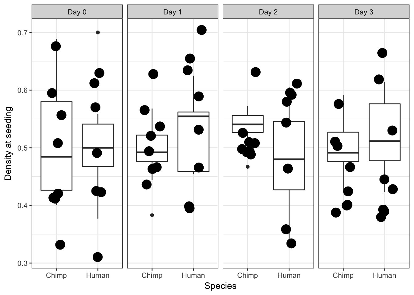

ggplot(data = iPSC_prop, aes(y = RIN_Score, x = as.factor(Species)))  + facet_wrap(~ Day, nrow = 1) + geom_boxplot()  + geom_dotplot(binaxis='y', stackdir='center', binwidth = 0.001) + labs(x = "Species", y = "Density at seeding") + theme_bw()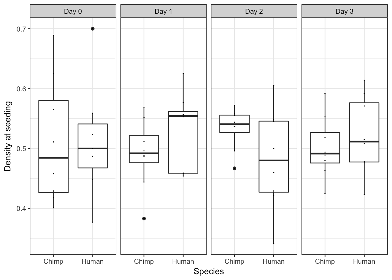

Harvest time and harvest densities (supplement)

iPSC_prop <- as.data.frame(cbind(day, species, RNA_seq_info[,9],  as.character(RNA_seq_info[,8])), stringsAsFactors = FALSE)

  
colnames(iPSC_prop) <- c("Day", "Species", "Harvest_density", "Harvest_time") 

iPSC_prop$Species[iPSC_prop$Species == "2"] <- "Human"
iPSC_prop$Species[iPSC_prop$Species == "1"] <- "Chimp"

iPSC_prop$Day[iPSC_prop$Day == "0"] <- "Day 0"
iPSC_prop$Day[iPSC_prop$Day == "1"] <- "Day 1"
iPSC_prop$Day[iPSC_prop$Day == "2"] <- "Day 2"
iPSC_prop$Day[iPSC_prop$Day == "3"] <- "Day 3"


iPSC_prop$Harvest_density <- as.numeric(iPSC_prop$Harvest_density)

ggplot(data = iPSC_prop, aes(y = Harvest_density, x = as.factor(Day)))  + facet_wrap(~ Species, nrow = 1) + geom_boxplot() + geom_point(aes(color = as.factor(Species)), size = 5,  position=position_jitter(width=0.2, height=0.1), show.legend = FALSE)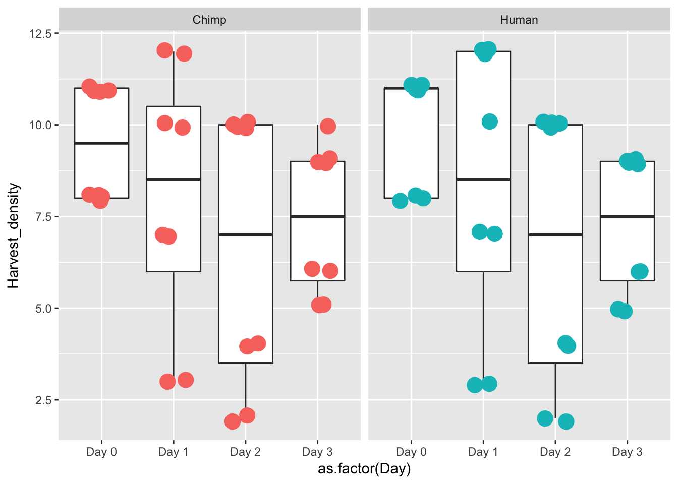

ggplot(data = iPSC_prop, aes(y = Harvest_density, x = as.factor(Species)))  + facet_wrap(~ Day, nrow = 1) + geom_boxplot()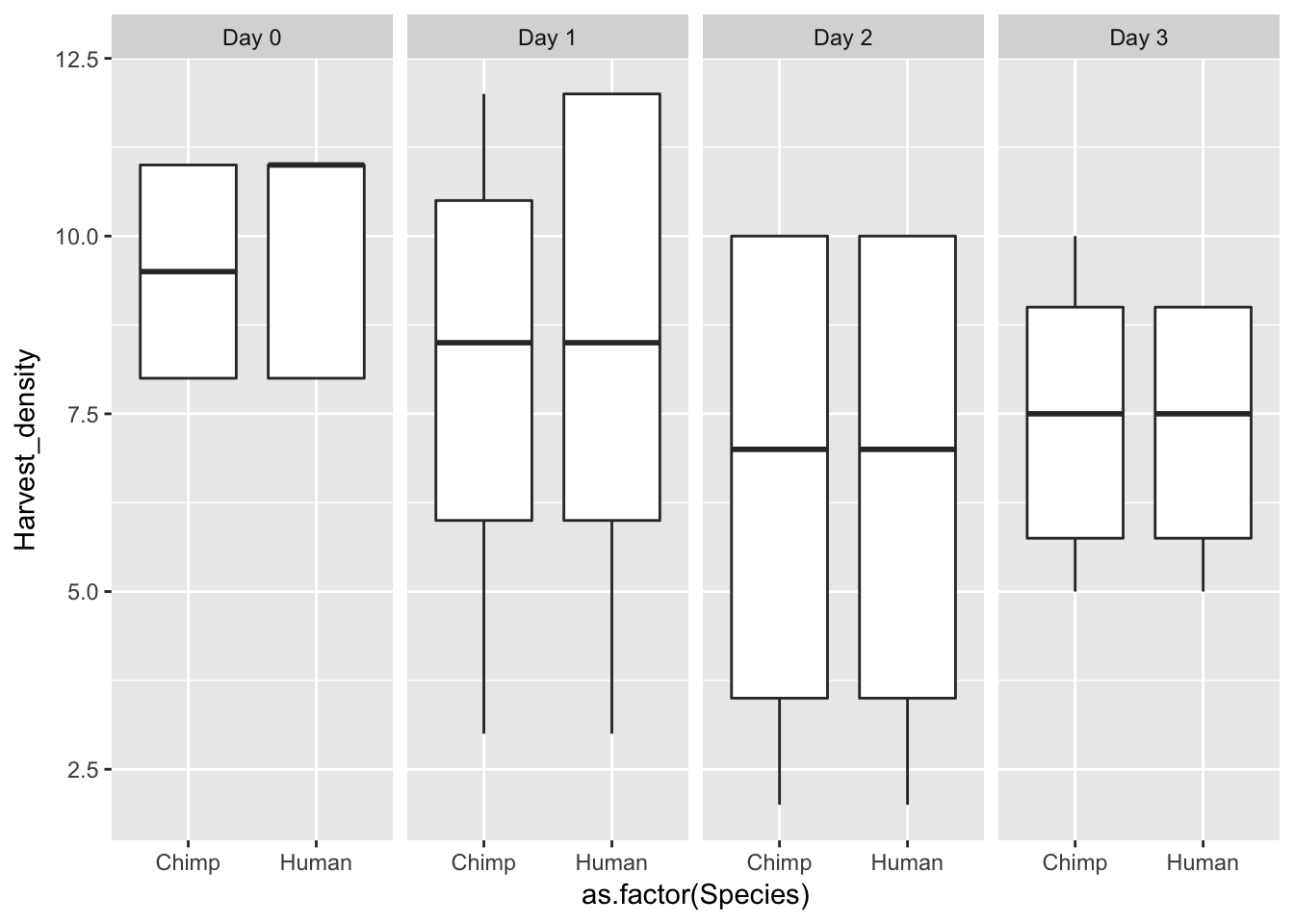

# Harvest density (supplement)

ggplot(data = iPSC_prop, aes(y = Harvest_density, x = Species))  + facet_wrap(~ Day, nrow = 1) + geom_boxplot() + geom_dotplot(binaxis='y', stackdir='center') + labs(y = "Harvest density", title = "Harvest densities for each sample") + theme_bw()

`stat_bindot()` using `bins = 30`. Pick better value with `binwidth`.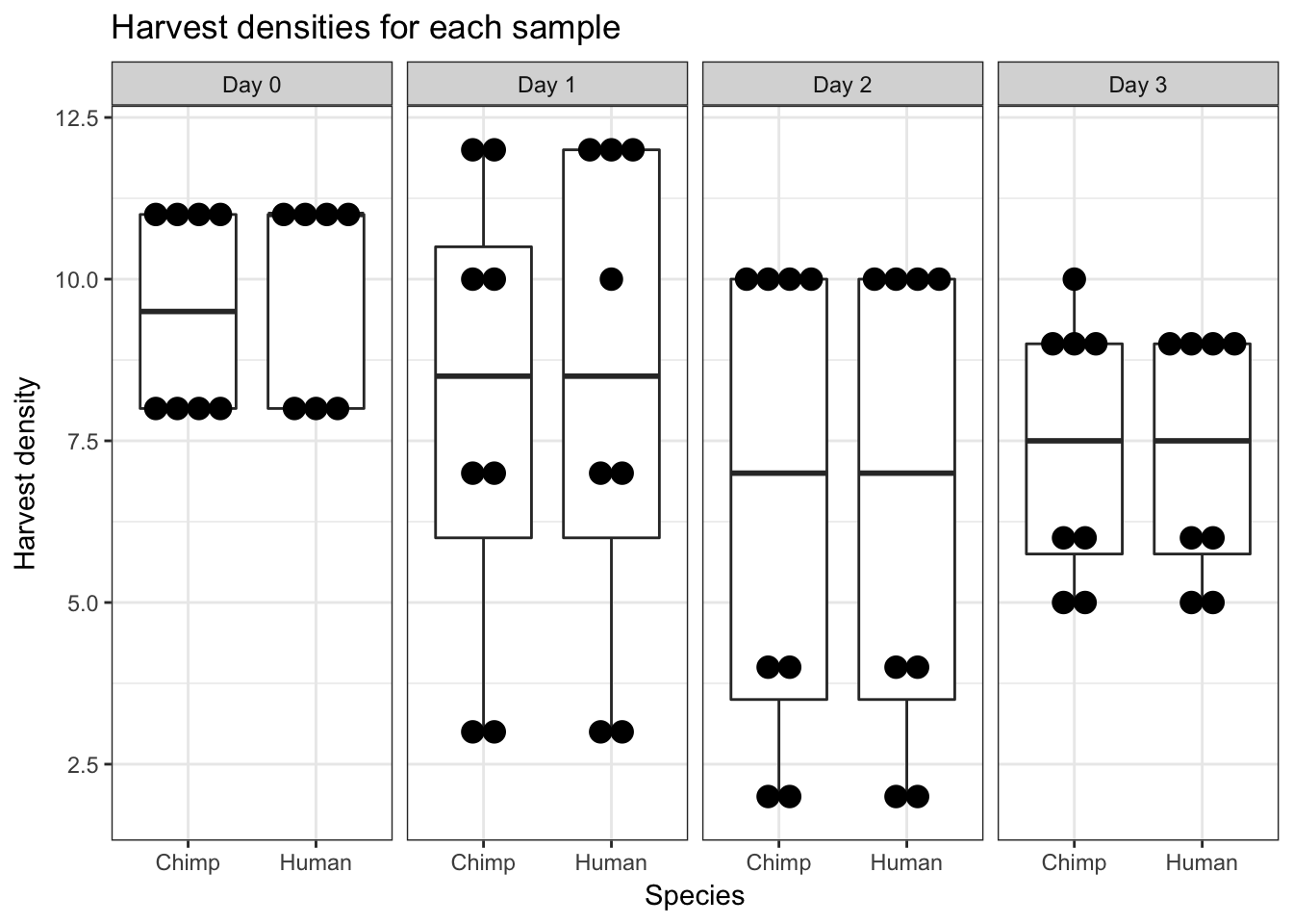

ggplot(data = iPSC_prop, aes(y = Harvest_density, x = Species))  + facet_wrap(~ Day, nrow = 1) + geom_boxplot() + geom_dotplot(binaxis='y', stackdir='center', dotsize = 0.75) + labs(y = "Harvest density", title = "Harvest densities for each sample") + theme_bw()

`stat_bindot()` using `bins = 30`. Pick better value with `binwidth`.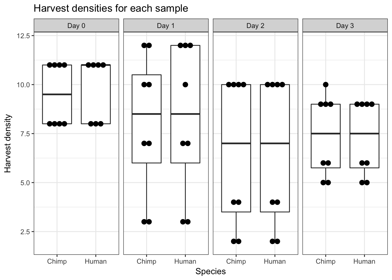

# Harvest density for each day species

median(iPSC_prop[which(iPSC_prop$Day == "Day 0" & iPSC_prop$Species == "human") , 3])

[1] NA

median(iPSC_prop[which(iPSC_prop$Day == "Day 0" & iPSC_prop$Species == "chimp") , 3])

[1] NA

median(iPSC_prop[which(iPSC_prop$Day == "Day 1" & iPSC_prop$Species == "human") , 3])

[1] NA

median(iPSC_prop[which(iPSC_prop$Day == "Day 1" & iPSC_prop$Species == "chimp") , 3])

[1] NA

median(iPSC_prop[which(iPSC_prop$Day == "Day 2" & iPSC_prop$Species == "human") , 3])

[1] NA

median(iPSC_prop[which(iPSC_prop$Day == "Day 2" & iPSC_prop$Species == "chimp") , 3])

[1] NA

median(iPSC_prop[which(iPSC_prop$Day == "Day 3" & iPSC_prop$Species == "human") , 3])

[1] NA

median(iPSC_prop[which(iPSC_prop$Day == "Day 3" & iPSC_prop$Species == "chimp") , 3])

[1] NA

# Harvest time

species <- After_removal_sample_info$Species
day <- After_removal_sample_info$Day

iPSC_prop <- as.data.frame(cbind(day, species, RNA_seq_info[,9],  as.character(RNA_seq_info[,8])), stringsAsFactors = FALSE)

colnames(iPSC_prop) <- c("Day", "Species", "Harvest_density", "Harvest_time") 

iPSC_prop$Species[iPSC_prop$Species == "2"] <- "Human"
iPSC_prop$Species[iPSC_prop$Species == "1"] <- "Chimp"

iPSC_prop$Day[iPSC_prop$Day == "0"] <- "Day 0"
iPSC_prop$Day[iPSC_prop$Day == "1"] <- "Day 1"
iPSC_prop$Day[iPSC_prop$Day == "2"] <- "Day 2"
iPSC_prop$Day[iPSC_prop$Day == "3"] <- "Day 3"

table(iPSC_prop$Day, iPSC_prop$Harvest_time)

       
        0.139242857 0.152871429 0.179485714 0.179771429 0.183085714
  Day 0           1           1           1           1           1
  Day 1           1           1           1           1           1
  Day 2           1           1           1           1           1
  Day 3           1           1           1           1           1
       
        0.195557143 0.201828571 0.228571429 0.233357143 0.267857143
  Day 0           1           1           1           1           1
  Day 1           1           1           2           1           1
  Day 2           1           1           2           1           1
  Day 3           1           1           2           1           1
       
        0.291428571 0.293714286 0.347142857 0.367857143
  Day 0           1           1           1           1
  Day 1           1           1           1           1
  Day 2           1           1           1           1
  Day 3           1           1           1           1

ggplot(data = iPSC_prop, aes(y = as.factor(Harvest_time), x = Species))  + facet_wrap(~ Day, nrow = 1)  + geom_point(aes(color = Species), size = 5,  position=position_jitter(width=0.2, height=0.1), show.legend = FALSE) + theme_bw()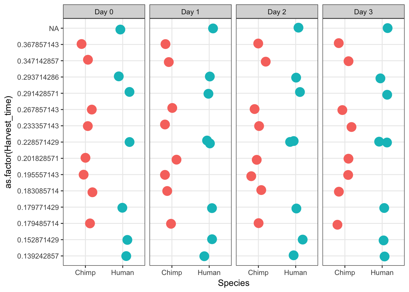

iPSC_prop[which(iPSC_prop$Day == "Day 0" & iPSC_prop$Species == "chimp") , 4]

character(0)

d0c <- table(factor(iPSC_prop[which(iPSC_prop$Day == "Day 0" & iPSC_prop$Species == "chimp") , 4], levels = c("11:56", "12:10", "12:18", "12:30", "1:00 PM", "1:05 PM", "1:06 PM", "1:08 PM", "1:17 PM", "1:20 PM", "1:30 PM")))

iPSC_prop[which(iPSC_prop$Day == "Day 0" & iPSC_prop$Species == "human") , 4]

character(0)

d0h <- table(factor(iPSC_prop[which(iPSC_prop$Day == "Day 0" & iPSC_prop$Species == "human") , 4], levels = c("11:56", "12:10", "12:18", "12:30", "1:00 PM", "1:05 PM", "1:06 PM", "1:08 PM", "1:17 PM", "1:20 PM", "1:30 PM")))

iPSC_prop[which(iPSC_prop$Day == "Day 1" & iPSC_prop$Species == "chimp") , 4]

character(0)

d1c <- table(factor(iPSC_prop[which(iPSC_prop$Day == "Day 1" & iPSC_prop$Species == "chimp") , 4], levels = c("11:56", "12:10", "12:18", "12:30", "1:00 PM", "1:05 PM", "1:06 PM", "1:08 PM", "1:17 PM", "1:20 PM", "1:30 PM")))

iPSC_prop[which(iPSC_prop$Day == "Day 1" & iPSC_prop$Species == "human") , 4]

character(0)

d1h <- table(factor(iPSC_prop[which(iPSC_prop$Day == "Day 1" & iPSC_prop$Species == "human") , 4], levels = c("11:56", "12:10", "12:18", "12:30", "1:00 PM", "1:05 PM", "1:06 PM", "1:08 PM", "1:17 PM", "1:20 PM", "1:30 PM")))

iPSC_prop[which(iPSC_prop$Day == "Day 2" & iPSC_prop$Species == "chimp") , 4]

character(0)

d2c <- table(factor(iPSC_prop[which(iPSC_prop$Day == "Day 2" & iPSC_prop$Species == "chimp") , 4], levels = c("11:56", "12:10", "12:18", "12:30", "1:00 PM", "1:05 PM", "1:06 PM", "1:08 PM", "1:17 PM", "1:20 PM", "1:30 PM")))

iPSC_prop[which(iPSC_prop$Day == "Day 2" & iPSC_prop$Species == "human") , 4]

character(0)

d2h <- table(factor(iPSC_prop[which(iPSC_prop$Day == "Day 2" & iPSC_prop$Species == "human") , 4], levels = c("11:56", "12:10", "12:18", "12:30", "1:00 PM", "1:05 PM", "1:06 PM", "1:08 PM", "1:17 PM", "1:20 PM", "1:30 PM")))

iPSC_prop[which(iPSC_prop$Day == "Day 3" & iPSC_prop$Species == "chimp") , 4]

character(0)

d3c <- table(factor(iPSC_prop[which(iPSC_prop$Day == "Day 3" & iPSC_prop$Species == "chimp") , 4], levels = c("11:56", "12:10", "12:18", "12:30", "1:00 PM", "1:05 PM", "1:06 PM", "1:08 PM", "1:17 PM", "1:20 PM", "1:30 PM")))

iPSC_prop[which(iPSC_prop$Day == "Day 3" & iPSC_prop$Species == "human") , 4]

character(0)

d3h <- table(factor(iPSC_prop[which(iPSC_prop$Day == "Day 3" & iPSC_prop$Species == "human") , 4], levels = c("11:56", "12:10", "12:18", "12:30", "1:00 PM", "1:05 PM", "1:06 PM", "1:08 PM", "1:17 PM", "1:20 PM", "1:30 PM")))

#Check that the frequencies match the input (n = 59)

frequency_time <- as.data.frame(cbind(d0c, d0h, d1c, d1h, d2c, d2h, d3c, d3h))

frequency_time

        d0c d0h d1c d1h d2c d2h d3c d3h
11:56     0   0   0   0   0   0   0   0
12:10     0   0   0   0   0   0   0   0
12:18     0   0   0   0   0   0   0   0
12:30     0   0   0   0   0   0   0   0
1:00 PM   0   0   0   0   0   0   0   0
1:05 PM   0   0   0   0   0   0   0   0
1:06 PM   0   0   0   0   0   0   0   0
1:08 PM   0   0   0   0   0   0   0   0
1:17 PM   0   0   0   0   0   0   0   0
1:20 PM   0   0   0   0   0   0   0   0
1:30 PM   0   0   0   0   0   0   0   0

plot(frequency_time[,1])

rowSums(frequency_time)

  11:56   12:10   12:18   12:30 1:00 PM 1:05 PM 1:06 PM 1:08 PM 1:17 PM 
      0       0       0       0       0       0       0       0       0 
1:20 PM 1:30 PM 
      0       0

# Order correctly

iPSC_prop$Harvest_time[iPSC_prop$Harvest_time == "11:56"] <- "11:56 AM"
iPSC_prop$Harvest_time[iPSC_prop$Harvest_time == "12:10"] <- "12:10 PM"
iPSC_prop$Harvest_time[iPSC_prop$Harvest_time == "12:18"] <- "12:18 PM"
iPSC_prop$Harvest_time[iPSC_prop$Harvest_time == "12:30"] <- "12:30 PM"

lv <- c("1:30 PM", "1:20 PM", "1:17 PM", "1:08 PM", "1:06 PM", "1:05 PM", "1:00 PM", "12:30 PM", "12:18 PM", "12:10 PM", "11:56 AM")
  
  
x <- factor(iPSC_prop$Harvest_time,levels = lv)

# Make plot

ggplot(data = iPSC_prop, aes(y = as.factor(x), x = as.factor(Species)))  + facet_wrap(~ Day, nrow = 1)  + geom_dotplot(binaxis='y', stackdir='center', binwidth = 0.2) + labs(x = "Species", y = "Harvest time") + theme_bw()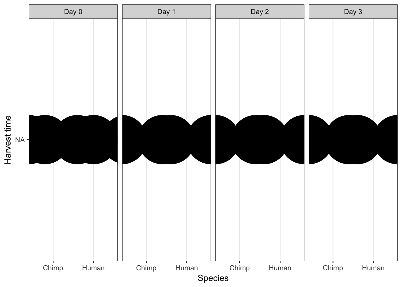

Purity

# Make a table with species, day, and RIN score
species <- After_removal_sample_info$Species
day <- After_removal_sample_info$Day

iPSC_prop <- as.data.frame(cbind(day, species, RNA_seq_info[,10]), stringsAsFactors = FALSE)

# Remove the samples with missing purity



iPSC_prop_purity <- iPSC_prop[complete.cases(iPSC_prop) == TRUE, ]

colnames(iPSC_prop_purity) <- c("Day", "Species", "Purity") 

iPSC_prop_purity$Species[iPSC_prop_purity$Species == "2"] <- "Human"
iPSC_prop_purity$Species[iPSC_prop_purity$Species == "1"] <- "Chimp"

iPSC_prop_purity$Day

 [1] 0 0 0 0 0 0 0 0 0 0 0 0 0 0 0 1 1 1 1 1 1 1 1 1 1 1 1 1 1 1 1 2 2 2 2
[36] 2 2 2 2 2 2 2 2 2 2 2 3 3 3 3 3 3 3 3 3 3 3 3 3 3 3

iPSC_prop_purity$Day[iPSC_prop_purity$Day == "0"] <- "Day 0"
iPSC_prop_purity$Day[iPSC_prop_purity$Day == "1"] <- "Day 1"
iPSC_prop_purity$Day[iPSC_prop_purity$Day == "2"] <- "Day 2"
iPSC_prop_purity$Day[iPSC_prop_purity$Day == "3"] <- "Day 3"

ggplot(data = iPSC_prop_purity, aes(y = Purity, x = as.factor(Species)))  + facet_wrap(~ Day, nrow = 1) + geom_boxplot() + geom_point(size = 5,  position=position_jitter(width=0.2, height=0.1), show.legend = FALSE) + labs(x = "Species", y = "Purity") + theme_bw()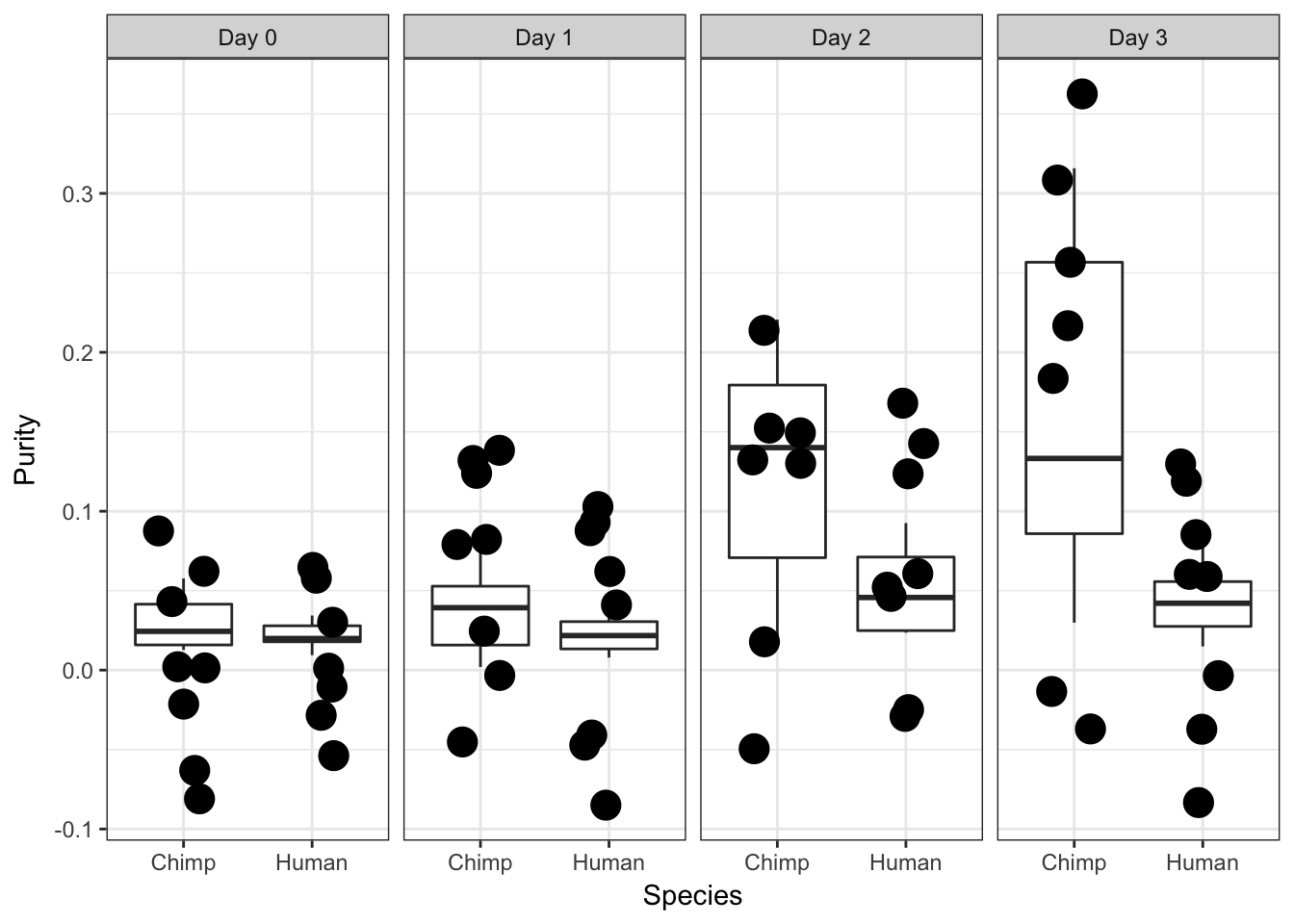

ggplot(data = iPSC_prop_purity, aes(y = Purity, x = as.factor(Species)))  + facet_wrap(~ Day, nrow = 1) + geom_boxplot() +  geom_dotplot(binaxis='y', stackdir='center', binwidth = .02) + labs(x = "Species", y = "Purity") + theme_bw()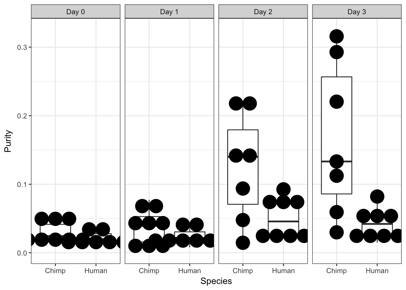

PART FOUR: See if any of the variables for RNA-Seq correlate with the expression PCs for genes (40 samples)

Initialization

# Load cpm data 

cpm_in_cutoff_40 <- read.delim("../data/cpm_cyclicloess_40.txt")

# Load sample information

bio_rep_samplefactors <- read.delim("../data/samplefactors-filtered.txt", stringsAsFactors=FALSE)
day <- bio_rep_samplefactors$Day
species <- bio_rep_samplefactors$Species

Obtain gene expression PCs (40 samples)

# PCs

pca_genes <- prcomp(t(cpm_in_cutoff_40), scale = T, retx = TRUE, center = TRUE)

matrixpca <- pca_genes$x
pc1 <- matrixpca[,1]
pc2 <- matrixpca[,2]
pc3 <- matrixpca[,3]
pc4 <- matrixpca[,4]
pc5 <- matrixpca[,5]

pcs <- data.frame(pc1, pc2, pc3, pc4, pc5)

summary <- summary(pca_genes)

Testing association between a particular variable and PCs with a linear model (40 samples)

# TESTING BIOLOGICAL VARIABLES OF INTEREST

PC_pvalues_day = matrix(data = NA, nrow = 5, ncol = 1, dimnames = list(c("PC1", "PC2", "PC3", "PC4", "PC5"), c("Day")))

for(i in 1:5){
# PC versus day

 checkPC1 <- lm(pcs[,i] ~ as.factor(day))

#Get the summary statistics from it
  summary(checkPC1)

#Get the p-value of the F-statistic
  summary(checkPC1)$fstatistic

  fstat <- as.data.frame(summary(checkPC1)$fstatistic)
  p_fstat <- 1-pf(fstat[1,], fstat[2,], fstat[3,])
  PC_pvalues_day[i,1] <- p_fstat
  
#Fraction of the variance explained by the model
  r2_value <- summary(checkPC1)$r.squared

}
# PC  versus species

PC_pvalues_species = matrix(data = NA, nrow = 5, ncol = 1, dimnames = list(c("PC1", "PC2", "PC3", "PC4", "PC5"), c("Species")))

for(i in 1:5){
# PC versus species

   checkPC1 <- lm(pcs[,i] ~ as.factor(species))

#Get the summary statistics from it
  summary(checkPC1)

#Get the p-value of the F-statistic
  summary(checkPC1)$fstatistic

  fstat <- as.data.frame(summary(checkPC1)$fstatistic)
  p_fstat <- 1-pf(fstat[1,], fstat[2,], fstat[3,])
  PC_pvalues_species [i,1] <- p_fstat 
  
#Fraction of the variance explained by the model
  r2_value <- summary(checkPC1)$r.squared
}

 # Combine tables

collapse_table_full <- rbind(PC_pvalues_day, PC_pvalues_species)

#Calculate q-values (FDR = 10%)

fdr_val = p.adjust(collapse_table_full, method = "fdr", n = length(collapse_table_full)*2)

collapse_table_fdr_val = matrix(data = fdr_val, nrow = 5, ncol = 2, dimnames = list(c("PC1", "PC2", "PC3", "PC4", "PC5"), c("Day", "Species")))

collapse_table_fdr_val

             Day   Species
PC1 0.000000e+00 0.4791868
PC2 1.000000e+00 0.0000000
PC3 1.494613e-08 0.8253925
PC4 1.670156e-01 0.9296140
PC5 5.072326e-01 1.0000000

Endoderm_TC_Technical_Factor_Analysis

Lauren Blake

January 12, 2017

PART ONE: See if any of the variables for RNA-Seq correlate with the expression PCs for genes (63 samples)

Initialization

Obtain gene expression PCs

Plots for PCs versus technical factors

Testing association between a particular variable and PCs with a linear model

Test for potential violations of the assumptions of the linear model

Find which factors are statistically significant

PART TWO: For the variable(s) that correlate, see if these segregate with either species or tissue

Testing to see if differences across variable groups are statistically significant for day.

Testing to see if differences across variable groups are statistically significant for species.

Find factors with FDR < 0.1

Combine and test day versus adapter for each sequencing pool

PART THREE: Which variables to consider putting in the model?

RIN Score

Passage at seed

Harvest time and harvest densities (supplement)

Purity

PART FOUR: See if any of the variables for RNA-Seq correlate with the expression PCs for genes (40 samples)

Initialization

Obtain gene expression PCs (40 samples)

Testing association between a particular variable and PCs with a linear model (40 samples)