Last updated: 2018-04-15

Code version: 5a57fa1

Introduction

Driving question: Are certain words more likely to be associated with “approved” applications and others with “non approved” words?

The following RMarkdown file uses files from Donors Choose and performs preliminary analysis with Latent Dirichlet allocation. The sentiment analysis was aided by the code and explanations provided in chapter 6 https://www.tidytextmining.com/.

Get Started

# Libraries

library(dplyr)


Attaching package: 'dplyr'

The following objects are masked from 'package:stats':

    filter, lag

The following objects are masked from 'package:base':

    intersect, setdiff, setequal, union

library(stringr)
library(tidytext)

Warning: package 'tidytext' was built under R version 3.4.4

library(ggplot2)
library(tidyverse)

── Attaching packages ────────────────────────────────────────────────────────────────────── tidyverse 1.2.1 ──

✔ tibble  1.4.2     ✔ readr   1.1.1
✔ tidyr   0.7.2     ✔ purrr   0.2.4
✔ tibble  1.4.2     ✔ forcats 0.2.0

── Conflicts ───────────────────────────────────────────────────────────────────────── tidyverse_conflicts() ──
✖ dplyr::filter() masks stats::filter()
✖ dplyr::lag()    masks stats::lag()

library("quanteda")

Warning: package 'quanteda' was built under R version 3.4.4

Package version: 1.1.1

Parallel computing: 2 of 8 threads used.

See https://quanteda.io for tutorials and examples.


Attaching package: 'quanteda'

The following object is masked from 'package:utils':

    View

library("plotly")


Attaching package: 'plotly'

The following object is masked from 'package:ggplot2':

    last_plot

The following object is masked from 'package:stats':

    filter

The following object is masked from 'package:graphics':

    layout

# Open the datasets

train <- read.csv("~/Dropbox/DonorsChoose/train.csv")
test <- read.csv("~/Dropbox/DonorsChoose/test.csv")
resources <- read.csv("~/Dropbox/DonorsChoose/resources.csv")

Make data into a tibble and find out the most common words in approved versus non-approved essays

# First, we want to select project id, essay 1, and if the project was approved or not

id_title <- c(1, 16, 10)

train_text <- train[,id_title]
train_text[,1] <- as.character(train_text[,1])
train_text[,2] <- as.numeric(train_text[,2])
train_text[,3] <- as.character(train_text[,3])


train_text <- as.tibble(train_text)

tidy_books <- train_text %>% unnest_tokens(word, project_essay_1)

# Take out stop (common) words

tidy_books <- tidy_books %>%
  anti_join(stop_words)

Joining, by = "word"

word_counts <- tidy_books %>%
  anti_join(stop_words) %>%
  count(id, word, sort = TRUE) %>%
  ungroup()

Joining, by = "word"

# Convert dtm

#chapters_dtm <- word_counts %>%
#  cast_dtm(id, word, n)

#chapters_dtm

# We have two topics (approved and not approved); set a seed so that the output of the model is predictable
#ap_lda <- LDA(chapters_dtm, k = 2, control = list(seed = 1234))

#topics <- tidy(ap_lda, matrix = "beta")

# Fnd the top words

#top_terms <- topics %>%
#  group_by(topic) %>%
#  top_n(5, beta) %>%
#  ungroup() %>%
#  arrange(topic, -beta)

#top_terms %>%
#  mutate(term = reorder(term, beta)) %>%
#  ggplot(aes(term, beta, fill = factor(topic))) +
#  geom_col(show.legend = FALSE) +
#  facet_wrap(~ topic, scales = "free") +
#  coord_flip()
# chapters_gamma <- tidy(ap_lda, matrix = "gamma")


# Look at frequency of different words


frequency <- tidy_books %>% 
  group_by(project_is_approved) %>% 
  count(word, sort = TRUE) %>% 
  left_join(tidy_books %>% 
              group_by(project_is_approved) %>% 
              summarise(total = n())) %>%
  mutate(freq = n/total)

Joining, by = "project_is_approved"

frequency <- frequency %>% 
  select(project_is_approved, word, freq) %>%
  spread(project_is_approved, freq)


library(scales)


Attaching package: 'scales'

The following object is masked from 'package:purrr':

    discard

The following object is masked from 'package:readr':

    col_factor

ggplot(frequency, aes(frequency[,2], frequency[,3])) +
  geom_jitter(alpha = 0.1, size = 2.5, width = 0.25, height = 0.25) +
  geom_text(aes(label = word), check_overlap = TRUE, vjust = 1.5) +
  scale_x_log10(labels = percent_format()) +
  scale_y_log10(labels = percent_format()) +
  geom_abline(color = "red")

Warning: Removed 26368 rows containing missing values (geom_point).

Warning: Removed 26368 rows containing missing values (geom_text).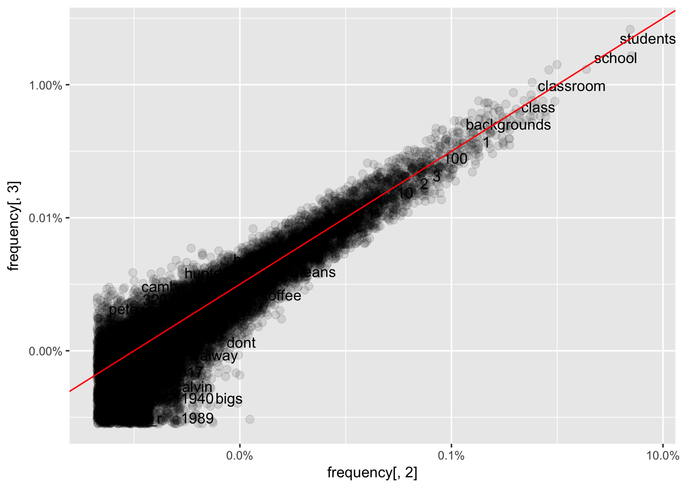

graph_associated_words <- function(min_freq){
word_ratios <- tidy_books %>%
  filter(!str_detect(word, "_")) %>%
  count(word, project_is_approved) 

word_ratios <- word_ratios[which(word_ratios$n > min_freq), ]

new_word_ratios <- word_ratios %>%
  ungroup() %>%
  spread(project_is_approved, n, fill = 0) %>%
  mutate_if(is.numeric, funs((. + 1) / sum(. + 1))) 

logratio <- log(new_word_ratios[,2] / new_word_ratios[,3])

new_word_ratios <- cbind(new_word_ratios, logratio)
colnames(new_word_ratios) <- c("word", "not_approved", "approved", "logratio")

#arrange_new_word_ratios <- new_word_ratios[order(new_word_ratios[,4]),] 

#arrange_new_word_ratios <- new_word_ratios[order(-new_word_ratios[,4]),] 

new_word_ratios %>% 
  arrange(abs(new_word_ratios[,4]))


new_word_ratios %>%
  group_by(logratio < 0) %>%
  top_n(15, abs(logratio)) %>%
  ungroup() %>%
  mutate(word = reorder(word, logratio)) %>%
  ggplot(aes(word, logratio, fill = logratio < 0)) +
  geom_col(show.legend = FALSE) +
  coord_flip() +
  ylab("log odds ratio (not approved/approved)") +
  scale_fill_discrete(name = "", labels = c("Not approved", "Approved"))

}

# Graph words associated with approved and not approved at different minimium frequencies
graph_associated_words(5000)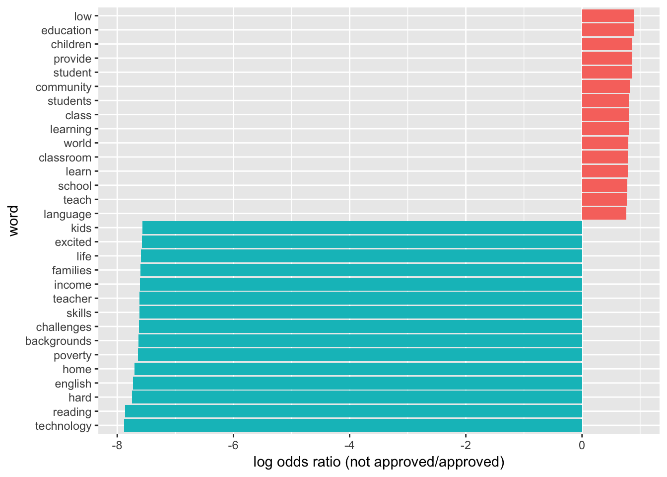

graph_associated_words(10000)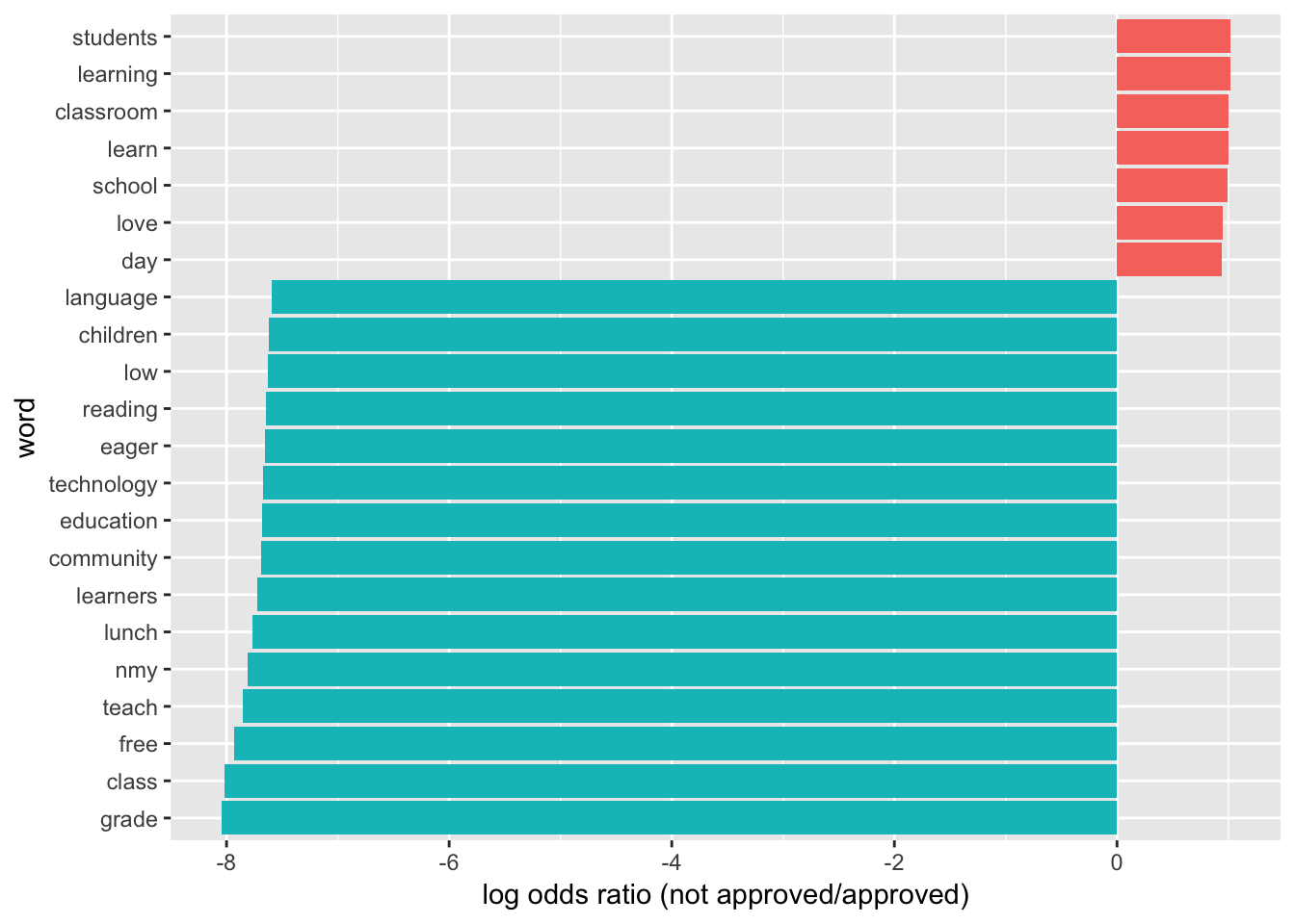

graph_associated_words(15000)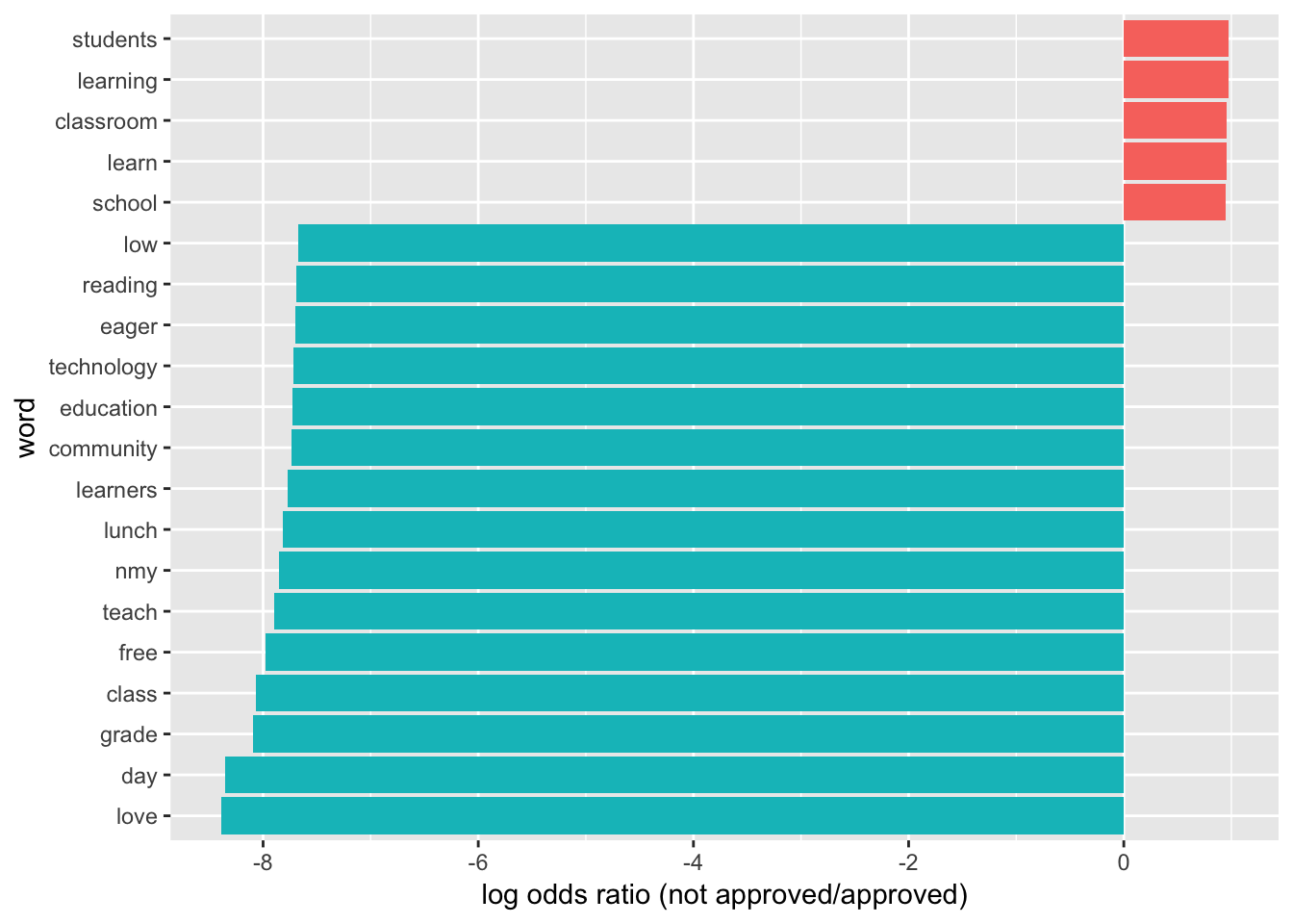

graph_associated_words(20000)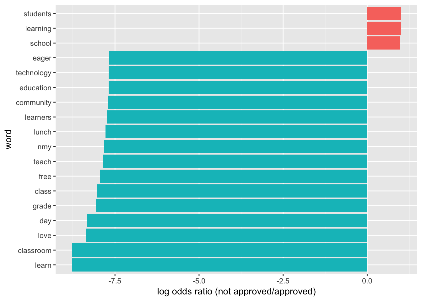

graph_associated_words(25000)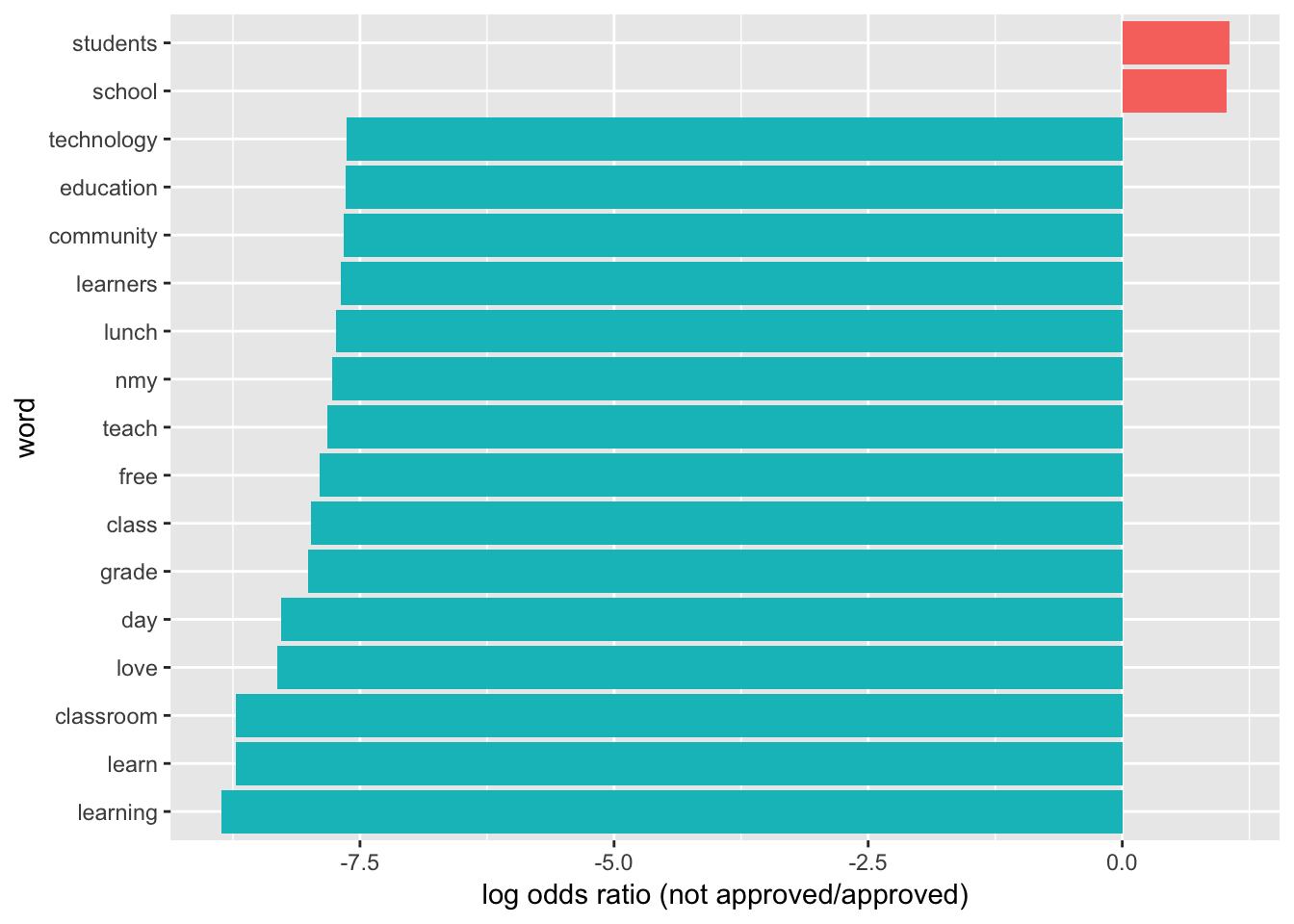

Which words in essay 1 are more likely to be associated with approval or not?

library(purrr)
library("ggrepel")

# Get frequency of words

frequency <- tidy_books %>% 
  group_by(project_is_approved) %>% 
  count(word, sort = TRUE) %>% 
  left_join(tidy_books %>% 
              group_by(project_is_approved) %>% 
              summarise(total = n())) %>%
  mutate(freq = n/total)

Joining, by = "project_is_approved"

# Select words that have been used at least 2000 times

frequency_50 <- frequency[which(frequency$n > 2000),]

frequency_50_0 <- frequency_50[which(frequency_50$project_is_approved != 1), ]
frequency_50_1 <- frequency_50[which(frequency_50$project_is_approved == 1), ]

appears_twice <- merge(frequency_50_0, frequency_50_1, by = c("word"))
dim(appears_twice)

[1] 99  9

ggplot(appears_twice, aes(freq.x, freq.y)) +
  geom_point(alpha = 0.8, size = 2.5, width = 0.25, height = 0.25) +
  geom_label_repel(aes(label = word)) +
  scale_x_log10(labels = percent_format()) +
  scale_y_log10(labels = percent_format()) +
  geom_abline(color = "red")

Warning: Ignoring unknown parameters: width, height

p <- ggplot(appears_twice, aes(freq.x, freq.y)) + 
  geom_point(aes(text = word), alpha = 0.8, size = 2.5, width = 0.25, height = 0.25)  +
  scale_x_log10(labels = percent_format()) +
  scale_y_log10(labels = percent_format()) +
  geom_abline(color = "red")

Warning: Ignoring unknown parameters: width, height

Warning: Ignoring unknown aesthetics: text

ggplotly(p)

We recommend that you use the dev version of ggplot2 with `ggplotly()`
Install it with: `devtools::install_github('hadley/ggplot2')`

Which words in essay 2 are more likely to be associated with approval?

id_title <- c(1, 16, 11)

train_text <- train[,id_title]
train_text[,1] <- as.character(train_text[,1])
train_text[,2] <- as.numeric(train_text[,2])
train_text[,3] <- as.character(train_text[,3])


train_text <- as.tibble(train_text)

tidy_books <- train_text %>% unnest_tokens(word, project_essay_2)

# Take out stop (common) words

tidy_books <- tidy_books %>%
  anti_join(stop_words)

Joining, by = "word"

word_counts <- tidy_books %>%
  anti_join(stop_words) %>%
  count(id, word, sort = TRUE) %>%
  ungroup()

Joining, by = "word"

frequency <- tidy_books %>% 
  group_by(project_is_approved) %>% 
  count(word, sort = TRUE) %>% 
  left_join(tidy_books %>% 
              group_by(project_is_approved) %>% 
              summarise(total = n())) %>%
  mutate(freq = n/total)

Joining, by = "project_is_approved"

# Select words that have been used at least 2000 times

frequency_50 <- frequency[which(frequency$n > 2000),]

frequency_50_0 <- frequency_50[which(frequency_50$project_is_approved != 1), ]
frequency_50_1 <- frequency_50[which(frequency_50$project_is_approved == 1), ]

appears_twice <- merge(frequency_50_0, frequency_50_1, by = c("word"))
dim(appears_twice)

[1] 104   9

ggplot(appears_twice, aes(freq.x, freq.y)) +
  geom_point(alpha = 0.8, size = 2.5, width = 0.25, height = 0.25) +
  geom_label_repel(aes(label = word)) +
  scale_x_log10(labels = percent_format()) +
  scale_y_log10(labels = percent_format()) +
  geom_abline(color = "red")

Warning: Ignoring unknown parameters: width, height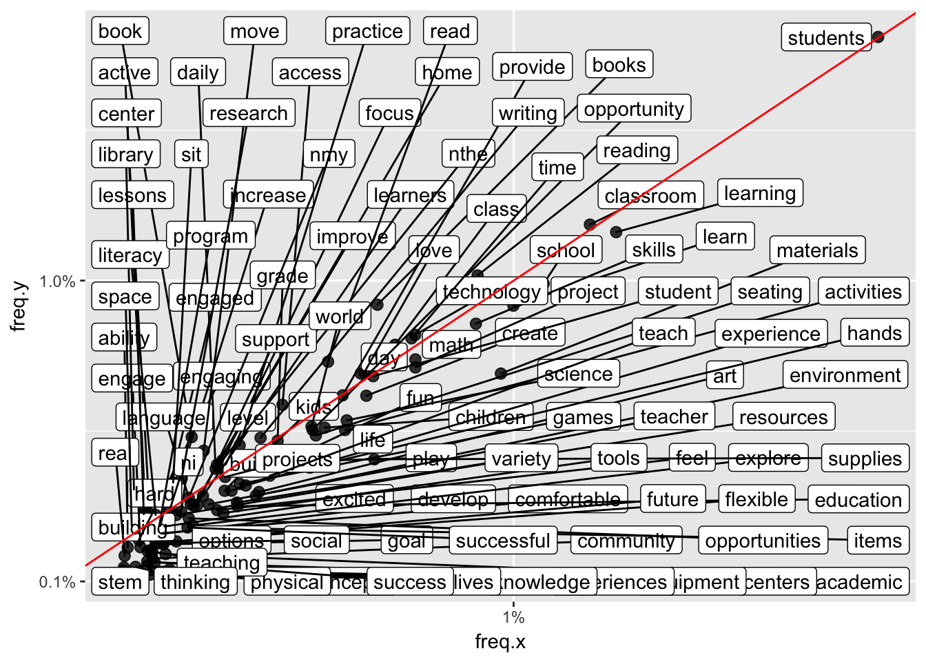

p <- ggplot(appears_twice, aes(freq.x, freq.y)) + 
  geom_point(aes(text = word), alpha = 0.8, size = 2.5, width = 0.25, height = 0.25)  +
  scale_x_log10(labels = percent_format()) +
  scale_y_log10(labels = percent_format()) +
  geom_abline(color = "red")

Warning: Ignoring unknown parameters: width, height

Warning: Ignoring unknown aesthetics: text

ggplotly(p)

We recommend that you use the dev version of ggplot2 with `ggplotly()`
Install it with: `devtools::install_github('hadley/ggplot2')`

Which resources are more likely to be associated with approval?

id_title <- c(1, 16, 14)

train_text <- train[,id_title]
train_text[,1] <- as.character(train_text[,1])
train_text[,2] <- as.numeric(train_text[,2])
train_text[,3] <- as.character(train_text[,3])


train_text <- as.tibble(train_text)

tidy_books <- train_text %>% unnest_tokens(word, project_resource_summary)

# Take out stop (common) words

tidy_books <- tidy_books %>%
  anti_join(stop_words)

Joining, by = "word"

word_counts <- tidy_books %>%
  anti_join(stop_words) %>%
  count(id, word, sort = TRUE) %>%
  ungroup()

Joining, by = "word"

frequency <- tidy_books %>% 
  group_by(project_is_approved) %>% 
  count(word, sort = TRUE) %>% 
  left_join(tidy_books %>% 
              group_by(project_is_approved) %>% 
              summarise(total = n())) %>%
  mutate(freq = n/total)

Joining, by = "project_is_approved"

summary(frequency$n)

     Min.   1st Qu.    Median      Mean   3rd Qu.      Max. 
     1.00      1.00      2.00     47.54      9.00 168279.00

# Select words that have been used at least 2000 times

frequency_50 <- frequency[which(frequency$n > 1500),]

frequency_50_0 <- frequency_50[which(frequency_50$project_is_approved != 1), ]
frequency_50_1 <- frequency_50[which(frequency_50$project_is_approved == 1), ]

appears_twice <- merge(frequency_50_0, frequency_50_1, by = c("word"))
dim(appears_twice)

[1] 17  9

ggplot(appears_twice, aes(freq.x, freq.y)) +
  geom_point(alpha = 0.8, size = 2.5, width = 0.25, height = 0.25) +
  geom_label_repel(aes(label = word)) +
  scale_x_log10(labels = percent_format()) +
  scale_y_log10(labels = percent_format()) +
  geom_abline(color = "red")

Warning: Ignoring unknown parameters: width, height

p <- ggplot(appears_twice, aes(freq.x, freq.y)) + 
  geom_point(aes(text = word), alpha = 0.8, size = 2.5, width = 0.25, height = 0.25)  +
  scale_x_log10(labels = percent_format()) +
  scale_y_log10(labels = percent_format()) +
  geom_abline(color = "red")

Warning: Ignoring unknown parameters: width, height

Warning: Ignoring unknown aesthetics: text

ggplotly(p)

We recommend that you use the dev version of ggplot2 with `ggplotly()`
Install it with: `devtools::install_github('hadley/ggplot2')`

Which titles are more likely to be associated with approval?

id_title <- c(1, 16, 9)

train_text <- train[,id_title]
train_text[,1] <- as.character(train_text[,1])
train_text[,2] <- as.numeric(train_text[,2])
train_text[,3] <- as.character(train_text[,3])


train_text <- as.tibble(train_text)

tidy_books <- train_text %>% unnest_tokens(word, project_title)

# Take out stop (common) words

tidy_books <- tidy_books %>%
  anti_join(stop_words)

Joining, by = "word"

word_counts <- tidy_books %>%
  anti_join(stop_words) %>%
  count(id, word, sort = TRUE) %>%
  ungroup()

Joining, by = "word"

frequency <- tidy_books %>% 
  group_by(project_is_approved) %>% 
  count(word, sort = TRUE) %>% 
  left_join(tidy_books %>% 
              group_by(project_is_approved) %>% 
              summarise(total = n())) %>%
  mutate(freq = n/total)

Joining, by = "project_is_approved"

summary(frequency$n)

    Min.  1st Qu.   Median     Mean  3rd Qu.     Max. 
    1.00     1.00     2.00    19.34     5.00 13114.00

# Select words that have been used at least 2000 times

frequency_50 <- frequency[which(frequency$n > 300),]

frequency_50_0 <- frequency_50[which(frequency_50$project_is_approved != 1), ]
frequency_50_1 <- frequency_50[which(frequency_50$project_is_approved == 1), ]

appears_twice <- merge(frequency_50_0, frequency_50_1, by = c("word"))
dim(appears_twice)

[1] 42  9

ggplot(appears_twice, aes(freq.x, freq.y)) +
  geom_point(alpha = 0.8, size = 2.5, width = 0.25, height = 0.25) +
  geom_label_repel(aes(label = word)) +
  scale_x_log10(labels = percent_format()) +
  scale_y_log10(labels = percent_format()) +
  geom_abline(color = "red")

Warning: Ignoring unknown parameters: width, height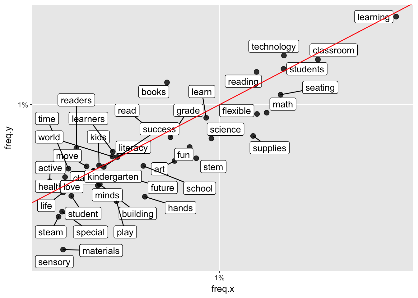

p <- ggplot(appears_twice, aes(freq.x, freq.y)) + 
  geom_point(aes(text = word), alpha = 0.8, size = 2.5, width = 0.25, height = 0.25)  +
  scale_x_log10(labels = percent_format()) +
  scale_y_log10(labels = percent_format()) +
  geom_abline(color = "red")

Warning: Ignoring unknown parameters: width, height

Warning: Ignoring unknown aesthetics: text

ggplotly(p)

We recommend that you use the dev version of ggplot2 with `ggplotly()`
Install it with: `devtools::install_github('hadley/ggplot2')`

Session information

sessionInfo()

R version 3.4.3 (2017-11-30)
Platform: x86_64-apple-darwin15.6.0 (64-bit)
Running under: OS X El Capitan 10.11.6

Matrix products: default
BLAS: /Library/Frameworks/R.framework/Versions/3.4/Resources/lib/libRblas.0.dylib
LAPACK: /Library/Frameworks/R.framework/Versions/3.4/Resources/lib/libRlapack.dylib

locale:
[1] en_US.UTF-8/en_US.UTF-8/en_US.UTF-8/C/en_US.UTF-8/en_US.UTF-8

attached base packages:
[1] stats     graphics  grDevices utils     datasets  methods   base     

other attached packages:
 [1] ggrepel_0.7.0   scales_0.5.0    bindrcpp_0.2    plotly_4.7.1   
 [5] quanteda_1.1.1  forcats_0.2.0   purrr_0.2.4     readr_1.1.1    
 [9] tidyr_0.7.2     tibble_1.4.2    tidyverse_1.2.1 ggplot2_2.2.1  
[13] tidytext_0.1.8  stringr_1.3.0   dplyr_0.7.4    

loaded via a namespace (and not attached):
 [1] Rcpp_0.12.15        lubridate_1.7.1     lattice_0.20-35    
 [4] assertthat_0.2.0    rprojroot_1.3-2     digest_0.6.15      
 [7] psych_1.7.8         mime_0.5            R6_2.2.2           
[10] cellranger_1.1.0    plyr_1.8.4          backports_1.1.2    
[13] evaluate_0.10.1     httr_1.3.1          pillar_1.1.0       
[16] rlang_0.1.6         lazyeval_0.2.1      readxl_1.0.0       
[19] rstudioapi_0.7      data.table_1.10.4-3 Matrix_1.2-13      
[22] rmarkdown_1.9       labeling_0.3        foreign_0.8-69     
[25] htmlwidgets_1.0     munsell_0.4.3       shiny_1.0.5        
[28] broom_0.4.3         httpuv_1.3.6.2      compiler_3.4.3     
[31] janeaustenr_0.1.5   spacyr_0.9.6        modelr_0.1.1       
[34] pkgconfig_2.0.1     mnormt_1.5-5        htmltools_0.3.6    
[37] tidyselect_0.2.3    viridisLite_0.3.0   crayon_1.3.4       
[40] SnowballC_0.5.1     grid_3.4.3          xtable_1.8-2       
[43] nlme_3.1-131        jsonlite_1.5        gtable_0.2.0       
[46] git2r_0.21.0        magrittr_1.5        tokenizers_0.2.0   
[49] RcppParallel_4.4.0  cli_1.0.0           stringi_1.1.7      
[52] reshape2_1.4.3      xml2_1.1.1          stopwords_0.9.0    
[55] fastmatch_1.1-0     tools_3.4.3         glue_1.2.0         
[58] crosstalk_1.0.0     hms_0.4.0           network_1.13.0.1   
[61] parallel_3.4.3      yaml_2.1.18         colorspace_1.3-2   
[64] rvest_0.3.2         knitr_1.20          bindr_0.1          
[67] haven_1.1.1

This R Markdown site was created with workflowr

Word frequency analysis

Lauren Blake

2018-04-06