Follow_up_best_set_tech_factors
Lauren Blake
August 9, 2016
Introduction
In the previous “Best set” analysis with tissue and species protected, we found that the following technical factors appeared in the best set for more than 2,400 of the 16,616 genes.
RNA Extraction date 3-23-12 (2nd technical factor on the design matrix fed into GLMnet). Note: the samples that have the RNA Extraction date of 3-23-12 are all Human Individual 3 samples (H3H, H3K, H3Li, H3Lu)
Mix code 1000 (8th technical factor). The chimp 1 liver (chimp 4x0519) is the only sample that has this multiplexing mix code because it was the only sample that was only in multiplex mix 1.
Percentage overlapping a junction (13th technical factor). Note: this was highest in reads mapped in livers than all of the other tissues. It does not appear to be confounded with species.
Reads mapped on orthologous exons (15th technical factor). Note: this was higher in liver and lung samples than heart and kidney samples. It does not appear to be confounded with species.
We have found confounders in the design (e.g. confounders with tissue and/or species). Now, we are looking to see if these confounders in the design are confounded with expression levels.
Exploratory Analysis
We want to see the distribution of expression values for the genes in which the best set contains one of the technical variables or not. Our original thought is that if the expression values for the genes in which the best set contains one of the technical variables are randomly distributed, then that is good and we probably won’t include it in the final model (used to determine DE genes). If the expression values for the genes in which the best set contains one of the technical variables are not randomly distributed, then we will consider including it in the final model when testing for DE genes.
# Load libraries

library("gplots")
##
## Attaching package: 'gplots'## The following object is masked from 'package:stats':
##
## lowesslibrary("ggplot2")
library("formattable")
# Load the data (biological and technical factors)
Best_set_bio_tech_var <- read.delim("~/Reg_Evo_Primates/ashlar-trial/data/Best_set_bio_tech_var.txt")
t_Best_set_bio_tech_var <- t(Best_set_bio_tech_var)
dim(t_Best_set_bio_tech_var)## [1] 16616 28# Load the data (expression counts data)
gene_counts_with_gc_correction <- read.delim("~/Reg_Evo_Primates/ashlar-trial/data/gc_cyclic_loess_random_var_gene_exp_counts")# Find average expression for each gene
chimp_hearts <- c(1, 5, 9, 13)
chimp_kidneys <- c(2,6,10,14)
chimp_livers <- c(3,7,11,15)
chimp_lungs <- c(4,8,12,16)
human_hearts <- c(20,24,28)
human_kidneys <- c(17,21,25,29)
human_livers <- c(18,22,26,30)
human_lungs <- c(19,23,27,31)
rhesus_hearts <- c(32,36,40,44)
rhesus_kidneys <- c(33,37,41,45)
rhesus_livers <- c(34,38,42,46)
rhesus_lungs <- c(35,39,43,47)
# For chimp hearts
exp_chimp_hearts <- as.data.frame(rowMeans(gene_counts_with_gc_correction[ , chimp_hearts]))
# For chimp kidneys
exp_chimp_kidneys <- as.data.frame(rowMeans(gene_counts_with_gc_correction[ , chimp_kidneys]))
# For chimp livers
exp_chimp_livers <- as.data.frame(rowMeans(gene_counts_with_gc_correction[ , chimp_livers]))
# For chimp lungs
exp_chimp_lungs <- as.data.frame(rowMeans(gene_counts_with_gc_correction[ , chimp_lungs]))
# For human hearts
exp_human_hearts <- as.data.frame(rowMeans(gene_counts_with_gc_correction[ , human_hearts]))
# For human kidneys
exp_human_kidneys <- as.data.frame(rowMeans(gene_counts_with_gc_correction[ , human_kidneys]))
# For human livers
exp_human_livers <- as.data.frame(rowMeans(gene_counts_with_gc_correction[ , human_livers]))
# For human lungs
exp_human_lungs <- as.data.frame(rowMeans(gene_counts_with_gc_correction[ , human_lungs]))
# For rhesus hearts
exp_rhesus_hearts <- as.data.frame(rowMeans(gene_counts_with_gc_correction[ , rhesus_hearts]))
# For rhesus kidneys
exp_rhesus_kidneys <- as.data.frame(rowMeans(gene_counts_with_gc_correction[ , rhesus_kidneys]))
# For rhesus livers
exp_rhesus_livers <- as.data.frame(rowMeans(gene_counts_with_gc_correction[ , rhesus_livers]))
# For rhesus lungs
exp_rhesus_lungs <- as.data.frame(rowMeans(gene_counts_with_gc_correction[ , human_lungs]))
# Make the data frame
avg_exp_values <- cbind(exp_chimp_hearts, exp_chimp_kidneys, exp_chimp_livers, exp_chimp_lungs, exp_human_hearts, exp_human_kidneys, exp_human_livers, exp_human_lungs, exp_rhesus_hearts, exp_rhesus_kidneys, exp_rhesus_livers, exp_rhesus_lungs)
rownames(avg_exp_values) <- row.names(gene_counts_with_gc_correction)
colnames(avg_exp_values) <- c("CH", "CK", "CLi", "CLu", "HH", "HK", "HLi", "HLu", "RH", "RK", "RLi", "RLu")
head(avg_exp_values)## CH CK CLi CLu HH HK
## ENSG00000000003 4.610868 6.396002 8.095469 5.391101 3.857809 6.931617
## ENSG00000000419 5.776325 5.204482 5.996511 5.432862 5.922276 5.660062
## ENSG00000000457 4.716621 5.185978 6.408613 5.111782 3.766371 4.320687
## ENSG00000000460 1.657578 1.692573 2.465693 2.189239 1.265669 2.309113
## ENSG00000000938 4.243727 3.971252 5.087452 7.650402 4.877109 3.562921
## ENSG00000000971 6.332304 5.125277 11.306291 6.282460 6.564142 5.757620
## HLi HLu RH RK RLi RLu
## ENSG00000000003 6.880175 4.857195 4.563435 7.071678 8.146930 4.857195
## ENSG00000000419 5.990137 5.463117 5.407861 5.223920 5.697787 5.463117
## ENSG00000000457 4.911001 4.272097 4.385651 5.077154 5.341901 4.272097
## ENSG00000000460 3.631794 2.487244 1.584310 1.547638 1.358645 2.487244
## ENSG00000000938 5.807408 7.568003 2.465641 2.432226 3.957756 7.568003
## ENSG00000000971 10.279503 7.651720 5.203002 6.511264 11.790392 7.651720# Add the 4 relevant technical variables
avg_exp_values_tech <- cbind(avg_exp_values, t_Best_set_bio_tech_var[,10], t_Best_set_bio_tech_var[,16], t_Best_set_bio_tech_var[,21], t_Best_set_bio_tech_var[,23], t_Best_set_bio_tech_var[,26])
colnames(avg_exp_values_tech) <- c("CH", "CK", "CLi", "CLu", "HH", "HK", "HLi", "HLu", "RH", "RK", "RLi", "RLu", "Extraction_3-23-12", "Mix_code_1000", "Perc_overlapping_junction", "Reads_mapped_on_ortho_exons", "RIN score")
# Check # of genes with technical variables
colSums(avg_exp_values_tech)## CH CK
## 55484.39 56037.61
## CLi CLu
## 56485.17 55182.71
## HH HK
## 55231.61 55509.20
## HLi HLu
## 56193.66 54984.79
## RH RK
## 55485.42 55221.47
## RLi RLu
## 56196.48 54984.79
## Extraction_3-23-12 Mix_code_1000
## 2511.00 2522.00
## Perc_overlapping_junction Reads_mapped_on_ortho_exons
## 3434.00 2425.00
## RIN score
## 1158.00# Put in a format ggplot2 likes
# All the tissue-species combinations
CH <- as.data.frame(rep("CH", times = 16616))
CK <- as.data.frame(rep("CK", times = 16616))
CLi <- as.data.frame(rep("CLi", times = 16616))
CLu <- as.data.frame(rep("CLu", times = 16616))
HH <- as.data.frame(rep("HH", times = 16616))
HK <- as.data.frame(rep("HK", times = 16616))
HLi <- as.data.frame(rep("HLi", times = 16616))
HLu <- as.data.frame(rep("HLu", times = 16616))
RH <- as.data.frame(rep("RH", times = 16616))
RK <- as.data.frame(rep("RK", times = 16616))
RLi <- as.data.frame(rep("RLi", times = 16616))
RLu <- as.data.frame(rep("RLu", times = 16616))
# Add expression and technical variables for each tissue-species combination
ggplot_avg_value_CH <- cbind(avg_exp_values_tech[,1], CH, avg_exp_values_tech[,13], avg_exp_values_tech[,14], avg_exp_values_tech[,15], avg_exp_values_tech[,16], avg_exp_values_tech[,17])
colnames(ggplot_avg_value_CH) <- c("Avg_Expression", "Sample", "RNA_Extra", "Mix_1000", "Perc_overlap_junct", "Reads_mapped_orth_exon", "RIN_Score")
ggplot_avg_value_CK <- cbind(avg_exp_values[,2], CK, avg_exp_values_tech[,13], avg_exp_values_tech[,14], avg_exp_values_tech[,15], avg_exp_values_tech[,16], avg_exp_values_tech[,17])
colnames(ggplot_avg_value_CK) <- colnames(ggplot_avg_value_CH)
ggplot_avg_value_CLi <- cbind(avg_exp_values[,3], CLi, avg_exp_values_tech[,13], avg_exp_values_tech[,14], avg_exp_values_tech[,15], avg_exp_values_tech[,16], avg_exp_values_tech[,17])
colnames(ggplot_avg_value_CLi) <- colnames(ggplot_avg_value_CH)
ggplot_avg_value_CLu <- cbind(avg_exp_values[,4], CLu, avg_exp_values_tech[,13], avg_exp_values_tech[,14], avg_exp_values_tech[,15], avg_exp_values_tech[,16], avg_exp_values_tech[,17])
colnames(ggplot_avg_value_CLu) <- colnames(ggplot_avg_value_CH)
ggplot_avg_value_HH <- cbind(avg_exp_values[,5], HH, avg_exp_values_tech[,13], avg_exp_values_tech[,14], avg_exp_values_tech[,15], avg_exp_values_tech[,16], avg_exp_values_tech[,17])
colnames(ggplot_avg_value_HH) <- colnames(ggplot_avg_value_CH)
ggplot_avg_value_HK <- cbind(avg_exp_values[,6], HK, avg_exp_values_tech[,13], avg_exp_values_tech[,14], avg_exp_values_tech[,15], avg_exp_values_tech[,16], avg_exp_values_tech[,17])
colnames(ggplot_avg_value_HK) <- colnames(ggplot_avg_value_CH)
ggplot_avg_value_HLi <- cbind(avg_exp_values[,7], HLi, avg_exp_values_tech[,13], avg_exp_values_tech[,14], avg_exp_values_tech[,15], avg_exp_values_tech[,16], avg_exp_values_tech[,17])
colnames(ggplot_avg_value_HLi) <- colnames(ggplot_avg_value_CH)
ggplot_avg_value_HLu <- cbind(avg_exp_values[,8], HLu, avg_exp_values_tech[,13], avg_exp_values_tech[,14], avg_exp_values_tech[,15], avg_exp_values_tech[,16], avg_exp_values_tech[,17])
colnames(ggplot_avg_value_HLu) <- colnames(ggplot_avg_value_CH)
ggplot_avg_value_RH <- cbind(avg_exp_values[,9], RH, avg_exp_values_tech[,13], avg_exp_values_tech[,14], avg_exp_values_tech[,15], avg_exp_values_tech[,16], avg_exp_values_tech[,17])
colnames(ggplot_avg_value_RH) <- colnames(ggplot_avg_value_CH)
ggplot_avg_value_RK <- cbind(avg_exp_values[,10], RK, avg_exp_values_tech[,13], avg_exp_values_tech[,14], avg_exp_values_tech[,15], avg_exp_values_tech[,16], avg_exp_values_tech[,17])
colnames(ggplot_avg_value_RK) <- colnames(ggplot_avg_value_CH)
ggplot_avg_value_RLi <- cbind(avg_exp_values[,11], RLi, avg_exp_values_tech[,13], avg_exp_values_tech[,14], avg_exp_values_tech[,15], avg_exp_values_tech[,16], avg_exp_values_tech[,17])
colnames(ggplot_avg_value_RLi) <- colnames(ggplot_avg_value_CH)
ggplot_avg_value_RLu <- cbind(avg_exp_values[,12], RLu, avg_exp_values_tech[,13], avg_exp_values_tech[,14], avg_exp_values_tech[,15], avg_exp_values_tech[,16], avg_exp_values_tech[,17])
colnames(ggplot_avg_value_RLu) <- colnames(ggplot_avg_value_CH)
# Combine all of the data frames
ggplot_avg_value <- rbind(ggplot_avg_value_CH, ggplot_avg_value_CK, ggplot_avg_value_CLi, ggplot_avg_value_CLu, ggplot_avg_value_HH, ggplot_avg_value_HK, ggplot_avg_value_HLi, ggplot_avg_value_HLu, ggplot_avg_value_RH, ggplot_avg_value_RK, ggplot_avg_value_RLi, ggplot_avg_value_RLu)
# Make labels
labels_RNA_Extra <- as.data.frame(paste(ggplot_avg_value$Sample, ggplot_avg_value$RNA_Extra, sep="_"))
colnames(labels_RNA_Extra) <- c("RNA_Extra_labels")
labels_Mix_1000 <- as.data.frame(paste(ggplot_avg_value$Sample, ggplot_avg_value$Mix_1000, sep="_"))
colnames(labels_Mix_1000) <- c("Mix_labels")
labels_Perc_overlap_junct <- as.data.frame(paste(ggplot_avg_value$Sample, ggplot_avg_value$Perc_overlap_junct, sep="_"))
colnames(labels_Perc_overlap_junct) <- c("Perc_overlap_junct_labels")
labels_Reads_mapped_orth_exon <- as.data.frame(paste(ggplot_avg_value$Sample, ggplot_avg_value$Reads_mapped_orth_exon, sep="_"))
colnames(labels_Reads_mapped_orth_exon) <- c("Reads_mapped_orth_exon_labels")
labels_RIN_Score <- as.data.frame(paste(ggplot_avg_value$Sample, ggplot_avg_value$RIN_Score, sep="_"))
colnames(labels_RIN_Score) <- c("RIN_Score_labels")
ggplot_avg_value_labels <- cbind(ggplot_avg_value, labels_RNA_Extra, labels_Mix_1000, labels_Perc_overlap_junct, labels_Reads_mapped_orth_exon, labels_RIN_Score)
# Make the plots
ggplot(ggplot_avg_value_labels, aes(factor(RNA_Extra_labels), Avg_Expression)) + geom_boxplot() + ylab("Normalized expression values (averaged over inds.)") + labs(title = "Expression values including genes with and without RNA Extraction Date 3-23-12") + xlab("Tissue-species + whether or not tech. factor included") + theme(axis.text.x = element_text(angle = 90, hjust = 1))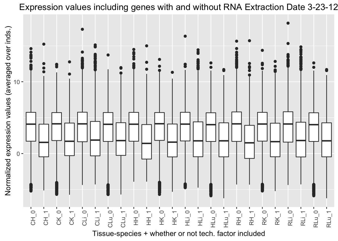
ggplot(ggplot_avg_value_labels, aes(factor(Mix_labels), Avg_Expression)) + geom_boxplot() + ylab("Normalized expression values (averaged over inds.)") + labs(title = "Expression values including genes with and without Master Mix Code 1000") + xlab("Tissue-species + whether or not tech. factor included") + theme(axis.text.x = element_text(angle = 90, hjust = 1))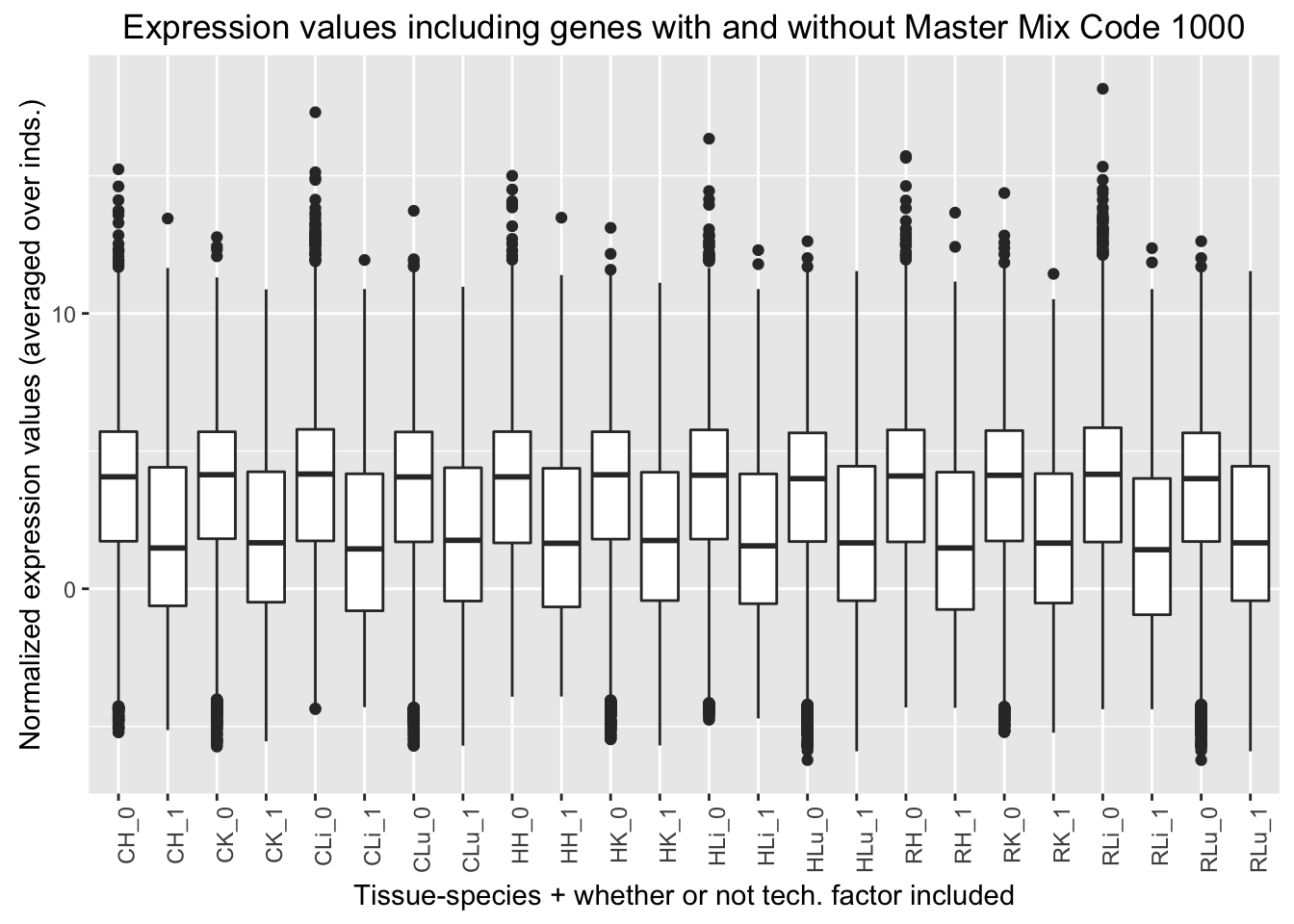
ggplot(ggplot_avg_value_labels, aes(factor(Perc_overlap_junct_labels), Avg_Expression)) + geom_boxplot() + ylab("Normalized expression values (averaged over inds.)") + labs(title = "Expression values including genes with and without Perc. overlapping junctions") + xlab("Tissue-species + whether or not tech. factor included") + theme(axis.text.x = element_text(angle = 90, hjust = 1))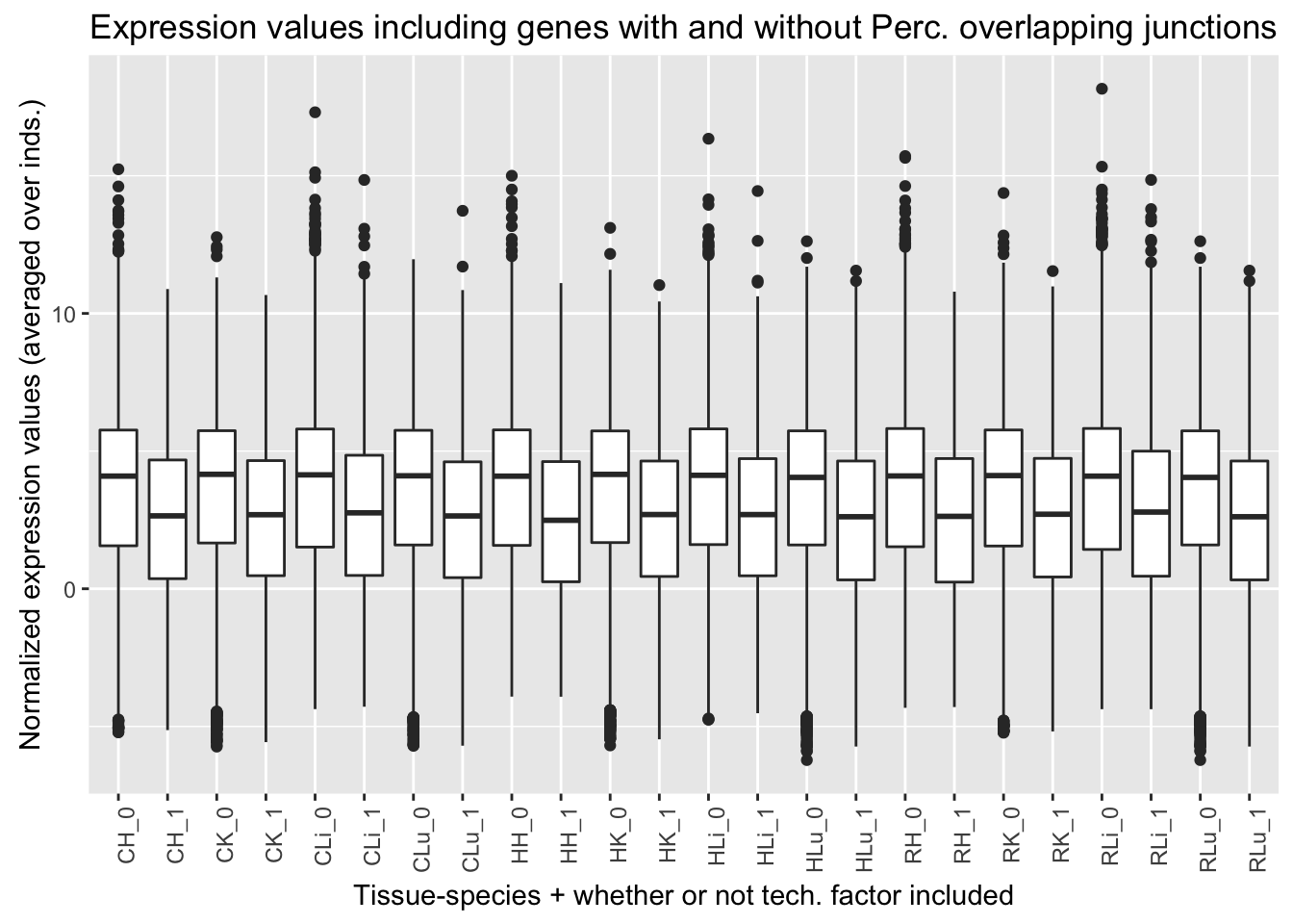
ggplot(ggplot_avg_value_labels, aes(factor(Reads_mapped_orth_exon_labels), Avg_Expression)) + geom_boxplot() + ylab("Normalized expression values (averaged over inds.)") + labs(title = "Expression values including genes with and without Num. of reads mapped on orth. exons") + xlab("Tissue-species + whether or not tech. factor included") + theme(axis.text.x = element_text(angle = 90, hjust = 1))
ggplot(ggplot_avg_value_labels, aes(factor(RIN_Score_labels), Avg_Expression)) + geom_boxplot() + ylab("Normalized expression values (averaged over inds.)") + labs(title = "Expression values including genes with and without RIN Score") + xlab("Tissue-species + whether or not tech. factor included") + theme(axis.text.x = element_text(angle = 90, hjust = 1))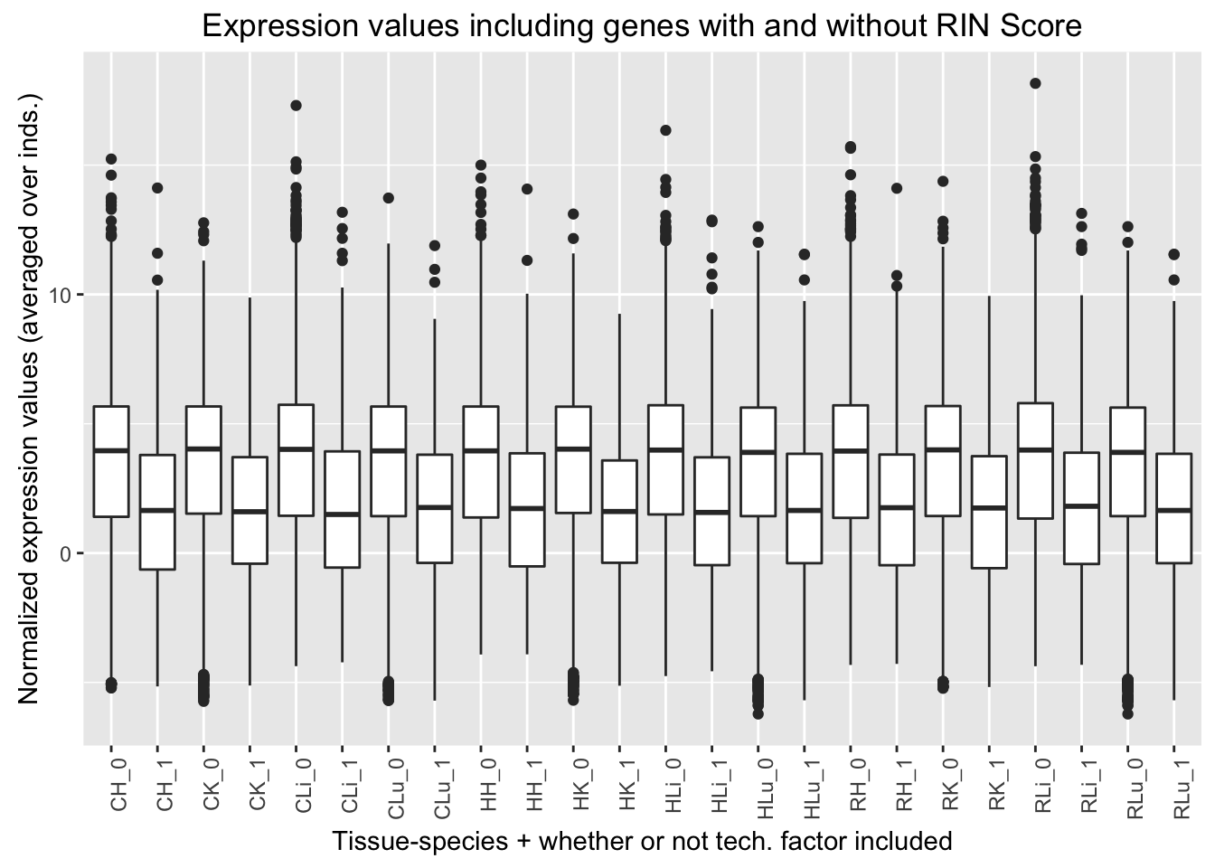
Determine if the technical factors are confounded with expression levels
We are going to determine if the averaged normalized expression values is the same or different for genes that have technical factor X included in the best set.
# Find the mean for all 47 samples
sample_means_per_gene <- rowMeans(gene_counts_with_gc_correction)

dim(sample_means_per_gene)
## NULL# Combine this with technical variables
exp_and_tech_var <- as.data.frame(cbind(sample_means_per_gene, avg_exp_values_tech[,13], avg_exp_values_tech[,14], avg_exp_values_tech[,15], avg_exp_values_tech[,16], avg_exp_values_tech[,17]))
colnames(exp_and_tech_var) <- c("Mean_all_samples", "Extraction_3_23_12", "Mix_code_1000", "Perc_overlapping_junction", "Reads_mapped_on_ortho_exons", "RIN_score")
dim(exp_and_tech_var)## [1] 16616 6# Find the quantiles of the means of all the samples
quantile(exp_and_tech_var$Mean_all_samples, probs = seq(0, 1, 0.25), na.rm = FALSE, names = TRUE, type = 7)## 0% 25% 50% 75% 100%
## -4.158937 1.329491 3.764888 5.471154 11.670442Q0 = -4.158937
Q1 = 1.329491
Q2 = 3.764888
Q3 = 5.471154
Q4 = 11.670442 Quantile analysis with RNA Extraction Date 3-21-16
# Find how many genes have 0 in the best set for RNA Extraction date 3-23-12 and which have 1 for each quantile

exp_RNA_extra_0_Q01 <- exp_and_tech_var[which(exp_and_tech_var$Extraction_3_23_12 == 0 & exp_and_tech_var$Mean_all_samples >= Q0 & exp_and_tech_var$Mean_all_samples < Q1 ), ]

dim(exp_RNA_extra_0_Q01)
## [1] 2966 6exp_RNA_extra_0_Q12 <- exp_and_tech_var[which(exp_and_tech_var$Extraction_3_23_12 == 0 & exp_and_tech_var$Mean_all_samples >= Q1 & exp_and_tech_var$Mean_all_samples < Q2 ), ]
dim(exp_RNA_extra_0_Q12)## [1] 3514 6exp_RNA_extra_0_Q23 <- exp_and_tech_var[which(exp_and_tech_var$Extraction_3_23_12 == 0 & exp_and_tech_var$Mean_all_samples >= Q2 & exp_and_tech_var$Mean_all_samples < Q3 ), ]
dim(exp_RNA_extra_0_Q23)## [1] 3759 6exp_RNA_extra_0_Q34 <- exp_and_tech_var[which(exp_and_tech_var$Extraction_3_23_12 == 0 & exp_and_tech_var$Mean_all_samples >= Q3 & exp_and_tech_var$Mean_all_samples < Q4 ), ]
dim(exp_RNA_extra_0_Q34)## [1] 3866 6exp_RNA_extra_1_Q01 <- exp_and_tech_var[which(exp_and_tech_var$Extraction_3_23_12 == 1 & exp_and_tech_var$Mean_all_samples >= Q0 & exp_and_tech_var$Mean_all_samples < Q1 ), ]
dim(exp_RNA_extra_1_Q01)## [1] 1188 6exp_RNA_extra_1_Q12 <- exp_and_tech_var[which(exp_and_tech_var$Extraction_3_23_12 == 1 & exp_and_tech_var$Mean_all_samples >= Q1 & exp_and_tech_var$Mean_all_samples < Q2 ), ]
dim(exp_RNA_extra_1_Q12)## [1] 640 6exp_RNA_extra_1_Q23 <- exp_and_tech_var[which(exp_and_tech_var$Extraction_3_23_12 == 1 & exp_and_tech_var$Mean_all_samples >= Q2 & exp_and_tech_var$Mean_all_samples < Q3 ), ]
dim(exp_RNA_extra_1_Q23)## [1] 395 6exp_RNA_extra_1_Q34 <- exp_and_tech_var[which(exp_and_tech_var$Extraction_3_23_12 == 1 & exp_and_tech_var$Mean_all_samples >= Q3 & exp_and_tech_var$Mean_all_samples < Q4 ), ]
dim(exp_RNA_extra_1_Q34)## [1] 288 6# Make a table of the values
DF <- data.frame(RNA_Extra_date_in_best_set=c("Yes", "No", "Ratio"), Q1=c("1188", "2966", "0.401"), Q2=c("640", "3514", "0.182"), Q3=c("395", "3759", "0.110"), Q4=c("288", "3866", "0.074"))
formattable(DF)| RNA_Extra_date_in_best_set | Q1 | Q2 | Q3 | Q4 |
|---|---|---|---|---|
| Yes | 1188 | 640 | 395 | 288 |
| No | 2966 | 3514 | 3759 | 3866 |
| Ratio | 0.401 | 0.182 | 0.110 | 0.074 |
Quantile analysis with Mix Code 1000
## [1] 2873 6## [1] 3583 6## [1] 3771 6## [1] 3867 6## [1] 1281 6## [1] 571 6## [1] 383 6## [1] 287 6| Mix_code_1000_in_best_set | Q1 | Q2 | Q3 | Q4 |
|---|---|---|---|---|
| Yes | 1281 | 571 | 383 | 287 |
| No | 2873 | 3583 | 3771 | 3867 |
| Ratio | 0.446 | 0.159 | 0.102 | 0.074 |
Quantile analysis with Percentage of reads overlapping a junction
## [1] 2912 6## [1] 3160 6## [1] 3445 6## [1] 3665 6## [1] 1242 6## [1] 994 6## [1] 709 6## [1] 489 6| Perc_overlapping_junction_in_best_set | Q1 | Q2 | Q3 | Q4 |
|---|---|---|---|---|
| Yes | 1242 | 994 | 709 | 489 |
| No | 2912 | 3160 | 3445 | 3665 |
| Ratio | 0.427 | 0.315 | 0.206 | 0.133 |
Quantile analysis with Number of reads mapped on orthologous exons
## [1] 3062 6## [1] 3499 6## [1] 3731 6## [1] 3899 6## [1] 1092 6## [1] 655 6## [1] 423 6## [1] 255 6| Perc_overlapping_junction_in_best_set | Q1 | Q2 | Q3 | Q4 |
|---|---|---|---|---|
| Yes | 1092 | 655 | 423 | 255 |
| No | 3062 | 3499 | 3731 | 3899 |
| Ratio | 0.357 | 0.187 | 0.113 | 0.065 |
Quantile analysis with RIN Score
## [1] 3573 6## [1] 3845 6## [1] 3958 6## [1] 4082 6## [1] 581 6## [1] 309 6## [1] 196 6## [1] 72 6| RNA_RIN_Score_in_best_set | Q1 | Q2 | Q3 | Q4 |
|---|---|---|---|---|
| Yes | 581 | 309 | 196 | 72 |
| No | 3573 | 3845 | 3958 | 4082 |
| Ratio | 0.163 | 0.080 | 0.050 | 0.018 |
Is average expression level correlated with number of technical factors included in the best set for each gene?
# Find the number of technical variables in the best set for each gene

num_tech_var <- as.data.frame(rowSums(t_Best_set_bio_tech_var)-7)
summary(num_tech_var)
## rowSums(t_Best_set_bio_tech_var) - 7
## Min. : 0.00
## 1st Qu.: 0.00
## Median : 1.00
## Mean : 1.68
## 3rd Qu.: 2.00
## Max. :12.00# Combine the number of technical variables in the best set for each gene with the mean expression level for each gene (over all 47 samples)
avg_exp_num_tech_var <- cbind(num_tech_var, exp_and_tech_var$Mean_all_samples)
colnames(avg_exp_num_tech_var) <- c("Num_tech_var", "Avg_Expression")
# Plot the results
ggplot(avg_exp_num_tech_var, aes(factor(Num_tech_var), Avg_Expression)) + geom_boxplot() + ylab("Normalized expression values (averaged over all inds.)") + labs(title = "Expression values versus technical factors in the best set") + xlab("Number of technical factors included in the best set analysis")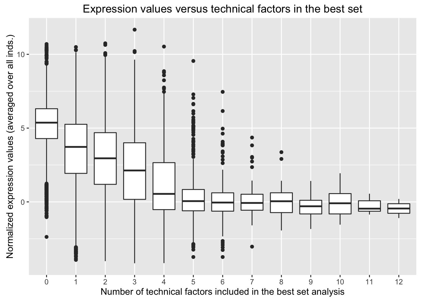
# The following code produces the same graph as above but the jitter function plots the actual points.

ggplot(avg_exp_num_tech_var, aes(factor(Num_tech_var), Avg_Expression)) + geom_boxplot() + geom_jitter() + ylab("Normalized expression values (averaged over all inds.)") + labs(title = "Expression values versus technical factors in the best set") + xlab("Number of technical factors included in the best set analysis") 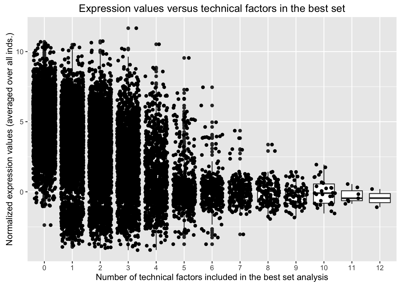
Conclusions: The number of technical factors identified in the best set is inversely proportional to the normalized expression values. I believe that the additional technical factors in the model may help to capture some of the noise around the lowly expressed genes. I think it is possible that this problem may be exacerbated by a relatively lax filtering strategy. Therefore, in the next set of analysis, I adopt a more stringent filtering strategy to see how this impacts the relationship between number of technical factors in the best set and expression values.