Introduction

The goal of this script is to identify the individuals that weight relapsed and the amount of change they underwent.

# Load libraries

library(ggplot2)

Warning: package 'ggplot2' was built under R version 3.4.4

library(cowplot)

Warning: package 'cowplot' was built under R version 3.4.4

Attaching package: 'cowplot'

The following object is masked from 'package:ggplot2':

    ggsave

# Get weight change data
weight_change <- read.csv("../data/weight_change.csv")

# Subset to time point 3

weight_change_t3 <- weight_change[weight_change$time == 3,]

summary(weight_change_t3)

     BAN_ID          time       Weight      Weight_change    
 Min.   :2201   Min.   :3   Min.   : 71.5   Min.   :-14.500  
 1st Qu.:2218   1st Qu.:3   1st Qu.:102.8   1st Qu.:  0.900  
 Median :2239   Median :3   Median :108.0   Median :  7.100  
 Mean   :2237   Mean   :3   Mean   :110.0   Mean   :  7.601  
 3rd Qu.:2256   3rd Qu.:3   3rd Qu.:118.4   3rd Qu.: 10.800  
 Max.   :2274   Max.   :3   Max.   :148.9   Max.   : 45.200  
                            NA's   :14      NA's   :14       
   Relapse_t3       Relapse_t4   Relapse_t5 
 Min.   :0.0000   Min.   :0    Min.   :0.0  
 1st Qu.:0.0000   1st Qu.:0    1st Qu.:0.0  
 Median :0.0000   Median :0    Median :0.5  
 Mean   :0.1951   Mean   :0    Mean   :0.5  
 3rd Qu.:0.0000   3rd Qu.:0    3rd Qu.:1.0  
 Max.   :1.0000   Max.   :0    Max.   :1.0  
 NA's   :14       NA's   :49   NA's   :49   

# How many are negative and how many are neutral/positive weight gain?

summary(weight_change_t3$Weight_change <0)

   Mode   FALSE    TRUE    NA's 
logical      33       8      14 

weight_change_t3[,5] <- weight_change_t3$Weight_change <0
colnames(weight_change_t3) <- c("BAN_ID", "time", "Weight", "Weight_change", "weight_relapse")

# Weight change from T2 to T3

weight_change_t3 <- weight_change_t3[complete.cases(weight_change_t3), ]
weight_change_t3_plot <- ggplot(weight_change_t3, aes(weight_relapse, Weight_change)) + geom_boxplot() + xlab("Lost weight from T2 to T3") + ylab("Weight change from T2 to T3")

save_plot("/Users/laurenblake/Dropbox/Figures/weight_change_t3.png", weight_change_t3_plot,          base_aspect_ratio = 1)

Weights over time, stratified by weight loss at T3

# Subset to time point 1

weight_change_t1 <- weight_change[weight_change$time == 1, 1:5]

# How many are negative and how many are neutral/positive weight gain?

summary(weight_change_t1$Relapse_t3 >0)

   Mode   FALSE    TRUE    NA's 
logical      33       8      14 

weight_change_t1[,6] <- weight_change_t1$Relapse_t3 >0
colnames(weight_change_t1) <- c("BAN_ID", "time", "Weight", "Weight_change", "Relapse_t3", "Relapse_notes")

weight_change_t1 <- weight_change_t1[complete.cases(weight_change_t1), ]

# Plot weight at T1 
weight_t1_plot <- ggplot(weight_change_t1, aes(Relapse_notes, Weight)) + geom_boxplot() + xlab("Lost weight from T2 to T3") + ylab("Weight") + ggtitle("Weight at T1") 

save_plot("/Users/laurenblake/Dropbox/Figures/weight_t1.png", weight_t1_plot,          base_aspect_ratio = 1)


# Subset to time point 2

weight_change_t1 <- weight_change[weight_change$time == 2, 1:5]

# How many are negative and how many are neutral/positive weight gain?

summary(weight_change_t1$Relapse_t3 >0)

   Mode   FALSE    TRUE    NA's 
logical      33       8      14 

weight_change_t1[,6] <- weight_change_t1$Relapse_t3 >0
colnames(weight_change_t1) <- c("BAN_ID", "time", "Weight", "Weight_change", "Relapse_t3", "Relapse_notes")

weight_change_t1 <- weight_change_t1[complete.cases(weight_change_t1), ]

# Plot weight at T1 
weight_t2_plot <- ggplot(weight_change_t1, aes(Relapse_notes, Weight)) + geom_boxplot() + xlab("Lost weight from T2 to T3") + ylab("Weight") + ggtitle("Weight at T2") + ylim(53,125)

save_plot("/Users/laurenblake/Dropbox/Figures/weight_t2.png", weight_t2_plot,          base_aspect_ratio = 1)


# Weight change from T1 to T2

weight_change_t1 <- weight_change_t1[complete.cases(weight_change_t1), ]
weight_change_t1_plot <- ggplot(weight_change_t1, aes(Relapse_notes, Weight_change)) + geom_boxplot() + xlab("Lost weight from T2 to T3") + ylab("Weight change from T1 to T2") + ylim(-15,46)

plot_grid(weight_change_t1_plot)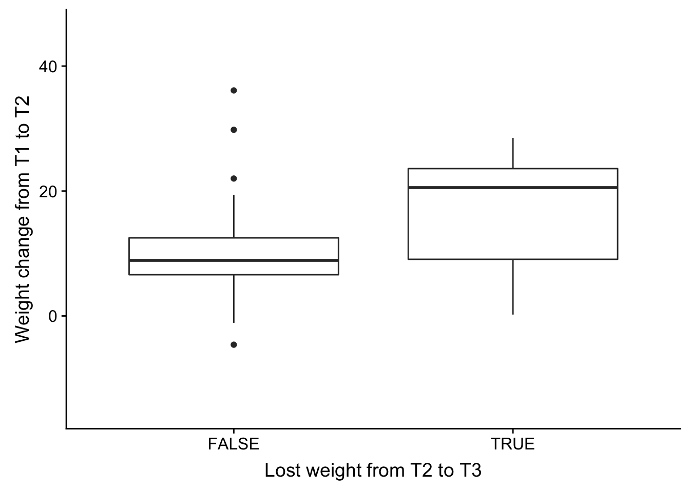

save_plot("/Users/laurenblake/Dropbox/Figures/weight_change_t1t2.png", weight_change_t1_plot,          base_aspect_ratio = 1)



# Subset to time point 3

weight_change_t1 <- weight_change[weight_change$time == 3, 1:5]

# How many are negative and how many are neutral/positive weight gain?

summary(weight_change_t1$Relapse_t3 >0)

   Mode   FALSE    TRUE    NA's 
logical      33       8      14 

weight_change_t1[,6] <- weight_change_t1$Relapse_t3 >0
colnames(weight_change_t1) <- c("BAN_ID", "time", "Weight", "Weight_change", "Relapse_t3", "Relapse_notes")

weight_change_t1 <- weight_change_t1[complete.cases(weight_change_t1), ]

# Plot weight at T1 
weight_t3_plot <- ggplot(weight_change_t1, aes(Relapse_notes, Weight)) + geom_boxplot() + xlab("Lost weight from T2 to T3") + ylab("Weight") + ggtitle("Weight at T3") + ylim(53,125)

save_plot("/Users/laurenblake/Dropbox/Figures/weight_t3.png", weight_t3_plot, base_aspect_ratio = 1)

Warning: Removed 6 rows containing non-finite values (stat_boxplot).

weight_change_t1_plot <- ggplot(weight_change_t1, aes(Relapse_notes, Weight_change)) + geom_boxplot() + xlab("Lost weight from T2 to T3") + ylab("Weight change from T2 to T3") + ylim(-15,46)

plot_grid(weight_change_t1_plot)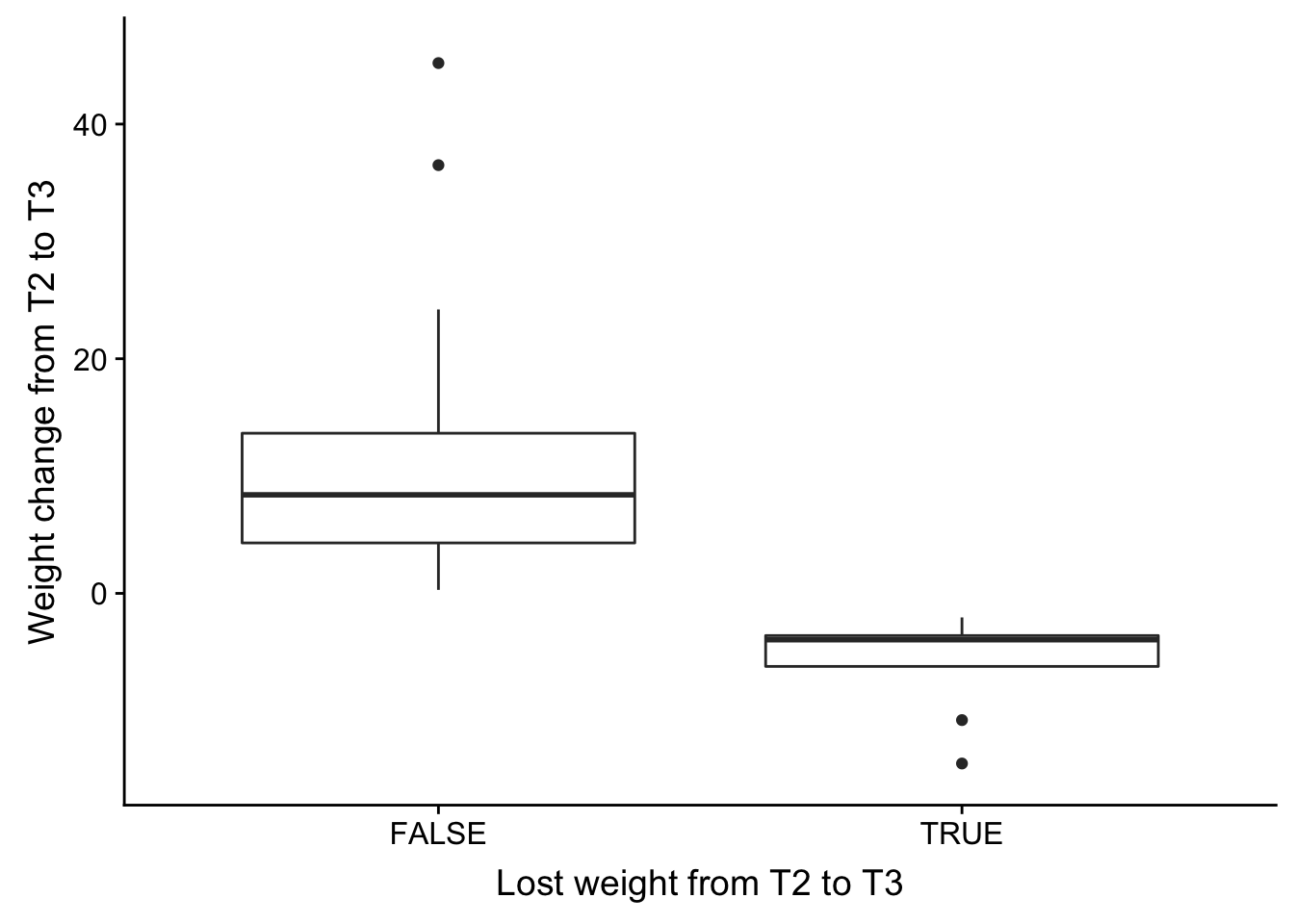

save_plot("/Users/laurenblake/Dropbox/Figures/weight_change_t2t3.png", weight_change_t1_plot,          base_aspect_ratio = 1)

Let’s look at the 8 individuals

# Let's look at the weight over time for the individuals with weight loss

weight_change_8 <- weight_change[weight_change$Relapse_t3 == 1,]

weight_change_8 <- weight_change_8[complete.cases(weight_change_8[,1:5]), ]

# Plot the individuals

ind_time <- ggplot(weight_change_8, aes(time, Weight, colour = as.factor(weight_change_8$BAN_ID))) + geom_point() + geom_line() + theme(legend.position="none") + xlab("Time")

plot_grid(ind_time)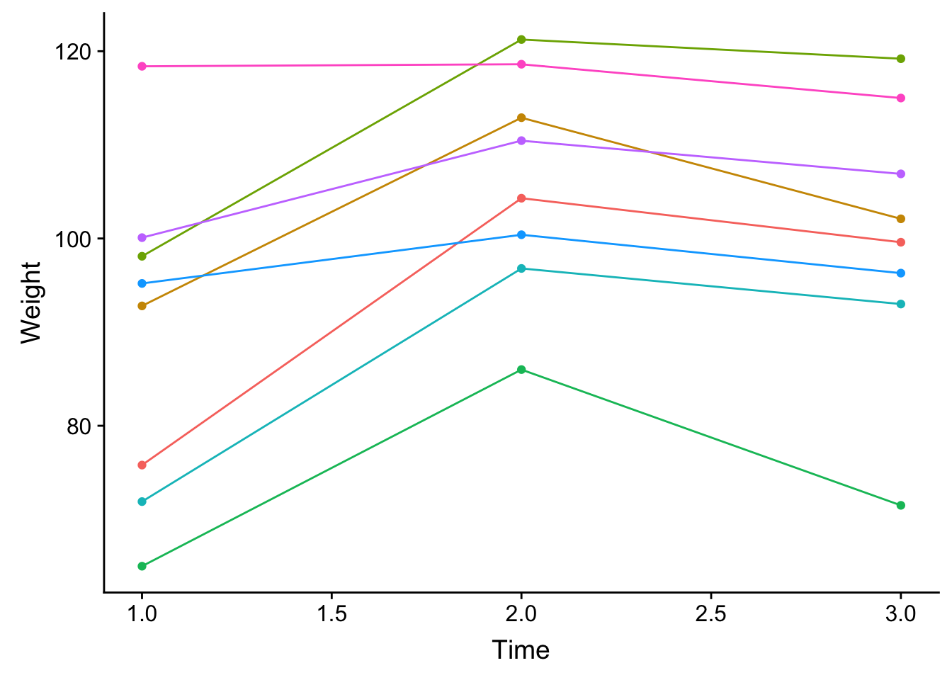

save_plot("/Users/laurenblake/Dropbox/Figures/weight_change_no_t3.png", ind_time,          base_aspect_ratio = 1)

# Summarize the 

weight_change_8_t3 <- weight_change_8[weight_change_8$time == 3,]

summary(weight_change_8_t3)

     BAN_ID          time       Weight       Weight_change    
 Min.   :2207   Min.   :3   Min.   : 71.50   Min.   :-14.500  
 1st Qu.:2226   1st Qu.:3   1st Qu.: 95.47   1st Qu.: -6.225  
 Median :2238   Median :3   Median :100.85   Median : -3.950  
 Mean   :2241   Mean   :3   Mean   :100.45   Mean   : -5.889  
 3rd Qu.:2262   3rd Qu.:3   3rd Qu.:108.92   3rd Qu.: -3.595  
 Max.   :2270   Max.   :3   Max.   :119.20   Max.   : -2.050  
                                                              
   Relapse_t3   Relapse_t4   Relapse_t5  
 Min.   :1    Min.   :0    Min.   :0.00  
 1st Qu.:1    1st Qu.:0    1st Qu.:0.25  
 Median :1    Median :0    Median :0.50  
 Mean   :1    Mean   :0    Mean   :0.50  
 3rd Qu.:1    3rd Qu.:0    3rd Qu.:0.75  
 Max.   :1    Max.   :0    Max.   :1.00  
              NA's   :6    NA's   :6     

Correlation between weight relapse and other variables

# Read in the clinical covariates

clinical_sample_info <- read.csv("../data/lm_covar_fixed_random.csv")
dim(clinical_sample_info)

[1] 156  14

# Subset to T1-T3

clinical_sample <- clinical_sample_info[1:144,(-12)]

dim(clinical_sample)

[1] 144  13

# Relapse 

chisq.test(as.factor(clinical_sample$Time), as.factor(clinical_sample$Relapse_t3), simulate.p.value = TRUE)$p.value

[1] 0.9585207

# Individual-yes

chisq.test(as.factor(clinical_sample$Individ), as.factor(clinical_sample$Relapse_t3), simulate.p.value = TRUE)$p.value

[1] 0.0004997501

# Age-yes
summary(lm(clinical_sample$Age ~ as.factor(clinical_sample$Relapse_t3)))

Call:
lm(formula = clinical_sample$Age ~ as.factor(clinical_sample$Relapse_t3))

Residuals:
   Min     1Q Median     3Q    Max 
-9.583 -5.583 -1.978  2.022 20.021 

Coefficients:
                                       Estimate Std. Error t value
(Intercept)                             23.9785     0.8045  29.806
as.factor(clinical_sample$Relapse_t3)1   6.6048     1.7763   3.718
                                       Pr(>|t|)    
(Intercept)                             < 2e-16 ***
as.factor(clinical_sample$Relapse_t3)1 0.000311 ***
---
Signif. codes:  0 '***' 0.001 '**' 0.01 '*' 0.05 '.' 0.1 ' ' 1

Residual standard error: 7.758 on 115 degrees of freedom
  (27 observations deleted due to missingness)
Multiple R-squared:  0.1073,    Adjusted R-squared:  0.09956 
F-statistic: 13.83 on 1 and 115 DF,  p-value: 0.0003114

# BE-no

chisq.test(as.factor(clinical_sample$BE_GROUP), as.factor(clinical_sample$Relapse_t3), simulate.p.value = TRUE)$p.value

[1] 0.4742629

# Psych meds- no

chisq.test(as.factor(clinical_sample$psychmeds), as.factor(clinical_sample$Relapse_t3), simulate.p.value = TRUE)$p.value

[1] 0.8270865

# RBC-no

summary(lm(clinical_sample$RBC ~ as.factor(clinical_sample$Relapse_t3)))

Call:
lm(formula = clinical_sample$RBC ~ as.factor(clinical_sample$Relapse_t3))

Residuals:
     Min       1Q   Median       3Q      Max 
-1.40750 -0.24763  0.02237  0.27237  1.22237 

Coefficients:
                                       Estimate Std. Error t value
(Intercept)                             4.22763    0.04503  93.883
as.factor(clinical_sample$Relapse_t3)1 -0.01013    0.09943  -0.102
                                       Pr(>|t|)    
(Intercept)                              <2e-16 ***
as.factor(clinical_sample$Relapse_t3)1    0.919    
---
Signif. codes:  0 '***' 0.001 '**' 0.01 '*' 0.05 '.' 0.1 ' ' 1

Residual standard error: 0.4343 on 115 degrees of freedom
  (27 observations deleted due to missingness)
Multiple R-squared:  9.034e-05, Adjusted R-squared:  -0.008605 
F-statistic: 0.01039 on 1 and 115 DF,  p-value: 0.919

# AE-no

summary(lm(clinical_sample$AE ~ as.factor(clinical_sample$Relapse_t3)))

Call:
lm(formula = clinical_sample$AE ~ as.factor(clinical_sample$Relapse_t3))

Residuals:
     Min       1Q   Median       3Q      Max 
-0.25833 -0.06344 -0.06344  0.03656  2.64167 

Coefficients:
                                       Estimate Std. Error t value
(Intercept)                             0.16344    0.02970   5.503
as.factor(clinical_sample$Relapse_t3)1  0.09489    0.06558   1.447
                                       Pr(>|t|)    
(Intercept)                            2.29e-07 ***
as.factor(clinical_sample$Relapse_t3)1    0.151    
---
Signif. codes:  0 '***' 0.001 '**' 0.01 '*' 0.05 '.' 0.1 ' ' 1

Residual standard error: 0.2864 on 115 degrees of freedom
  (27 observations deleted due to missingness)
Multiple R-squared:  0.01788,   Adjusted R-squared:  0.009343 
F-statistic: 2.094 on 1 and 115 DF,  p-value: 0.1506

# Race- no

chisq.test(as.factor(clinical_sample$Race), as.factor(clinical_sample$Relapse_t3), simulate.p.value = TRUE)$p.value

[1] 0.4582709

# AL- no

summary(lm(clinical_sample$AL ~ as.factor(clinical_sample$Relapse_t3)))

Call:
lm(formula = clinical_sample$AL ~ as.factor(clinical_sample$Relapse_t3))

Residuals:
     Min       1Q   Median       3Q      Max 
-1.11505 -0.41505 -0.01505  0.48495  1.38495 

Coefficients:
                                       Estimate Std. Error t value
(Intercept)                             1.81505    0.05936  30.580
as.factor(clinical_sample$Relapse_t3)1 -0.11505    0.13105  -0.878
                                       Pr(>|t|)    
(Intercept)                              <2e-16 ***
as.factor(clinical_sample$Relapse_t3)1    0.382    
---
Signif. codes:  0 '***' 0.001 '**' 0.01 '*' 0.05 '.' 0.1 ' ' 1

Residual standard error: 0.5724 on 115 degrees of freedom
  (27 observations deleted due to missingness)
Multiple R-squared:  0.006657,  Adjusted R-squared:  -0.00198 
F-statistic: 0.7707 on 1 and 115 DF,  p-value: 0.3818

# AN- no

summary(lm(clinical_sample$AN ~ as.factor(clinical_sample$Relapse_t3)))

Call:
lm(formula = clinical_sample$AN ~ as.factor(clinical_sample$Relapse_t3))

Residuals:
    Min      1Q  Median      3Q     Max 
-2.2258 -0.9258 -0.3258  0.5742  4.5500 

Coefficients:
                                       Estimate Std. Error t value
(Intercept)                              3.0258     0.1282  23.607
as.factor(clinical_sample$Relapse_t3)1   0.2242     0.2830   0.792
                                       Pr(>|t|)    
(Intercept)                              <2e-16 ***
as.factor(clinical_sample$Relapse_t3)1     0.43    
---
Signif. codes:  0 '***' 0.001 '**' 0.01 '*' 0.05 '.' 0.1 ' ' 1

Residual standard error: 1.236 on 115 degrees of freedom
  (27 observations deleted due to missingness)
Multiple R-squared:  0.005428,  Adjusted R-squared:  -0.003221 
F-statistic: 0.6276 on 1 and 115 DF,  p-value: 0.4299

# RIN- no

summary(lm(clinical_sample$RIN ~ as.factor(clinical_sample$Relapse_t3)))

Call:
lm(formula = clinical_sample$RIN ~ as.factor(clinical_sample$Relapse_t3))

Residuals:
     Min       1Q   Median       3Q      Max 
-2.37742 -0.27742  0.02258  0.42258  1.22258 

Coefficients:
                                       Estimate Std. Error t value
(Intercept)                             6.67742    0.07043  94.809
as.factor(clinical_sample$Relapse_t3)1 -0.10659    0.15551  -0.685
                                       Pr(>|t|)    
(Intercept)                              <2e-16 ***
as.factor(clinical_sample$Relapse_t3)1    0.494    
---
Signif. codes:  0 '***' 0.001 '**' 0.01 '*' 0.05 '.' 0.1 ' ' 1

Residual standard error: 0.6792 on 115 degrees of freedom
  (27 observations deleted due to missingness)
Multiple R-squared:  0.004069,  Adjusted R-squared:  -0.004592 
F-statistic: 0.4698 on 1 and 115 DF,  p-value: 0.4945

sessionInfo()

R version 3.4.3 (2017-11-30)
Platform: x86_64-apple-darwin15.6.0 (64-bit)
Running under: OS X El Capitan 10.11.6

Matrix products: default
BLAS: /Library/Frameworks/R.framework/Versions/3.4/Resources/lib/libRblas.0.dylib
LAPACK: /Library/Frameworks/R.framework/Versions/3.4/Resources/lib/libRlapack.dylib

locale:
[1] en_US.UTF-8/en_US.UTF-8/en_US.UTF-8/C/en_US.UTF-8/en_US.UTF-8

attached base packages:
[1] stats     graphics  grDevices utils     datasets  methods   base     

other attached packages:
[1] cowplot_0.9.3 ggplot2_3.0.0

loaded via a namespace (and not attached):
 [1] Rcpp_0.12.18      compiler_3.4.3    pillar_1.3.0     
 [4] git2r_0.23.0      plyr_1.8.4        workflowr_1.1.1  
 [7] bindr_0.1.1       R.methodsS3_1.7.1 R.utils_2.7.0    
[10] tools_3.4.3       digest_0.6.16     evaluate_0.11    
[13] tibble_1.4.2      gtable_0.2.0      pkgconfig_2.0.2  
[16] rlang_0.2.2       yaml_2.2.0        bindrcpp_0.2.2   
[19] withr_2.1.2       stringr_1.3.1     dplyr_0.7.6      
[22] knitr_1.20        rprojroot_1.3-2   grid_3.4.3       
[25] tidyselect_0.2.4  glue_1.3.0        R6_2.2.2         
[28] rmarkdown_1.10    purrr_0.2.5       magrittr_1.5     
[31] whisker_0.3-2     backports_1.1.2   scales_1.0.0     
[34] htmltools_0.3.6   assertthat_0.2.0  colorspace_1.3-2 
[37] labeling_0.3      stringi_1.2.4     lazyeval_0.2.1   
[40] munsell_0.5.0     crayon_1.3.4      R.oo_1.22.0