voom_limma_hg37

Introduction

# Library

library(edgeR)

Loading required package: limma

library(limma)
library(VennDiagram)

Warning: package 'VennDiagram' was built under R version 3.4.4

Loading required package: grid

Loading required package: futile.logger

library(cowplot)

Warning: package 'cowplot' was built under R version 3.4.4

Loading required package: ggplot2

Warning: package 'ggplot2' was built under R version 3.4.4

Attaching package: 'cowplot'

The following object is masked from 'package:ggplot2':

    ggsave

# Read in the data

tx.salmon <- readRDS("../data/counts_hg37_gc_txsalmon.RData")
salmon_counts<- as.data.frame(tx.salmon$counts)


#tx.salmon <- readRDS("../data/counts_hg38_gc_dds.RData")
#salmon_counts<- as.data.frame(tx.salmon)


# Subset to T1-T3

salmon_counts <- salmon_counts[,1:144]

# Read in the clinical covariates

clinical_sample_info <- read.csv("../data/lm_covar_fixed_random.csv")
dim(clinical_sample_info)

[1] 156  14

# Subset to T1-T3

clinical_sample <- clinical_sample_info[1:144,(-12)]

dim(clinical_sample)

[1] 144  13

Differential expression pipeline

# Filter lowly expressed reads

cpm <- cpm(salmon_counts, log=TRUE)

expr_cutoff <- 1.5
hist(cpm, main = "log2(CPM) values in unfiltered data", breaks = 100, xlab = "log2(CPM) values")
abline(v = expr_cutoff, col = "red", lwd = 3)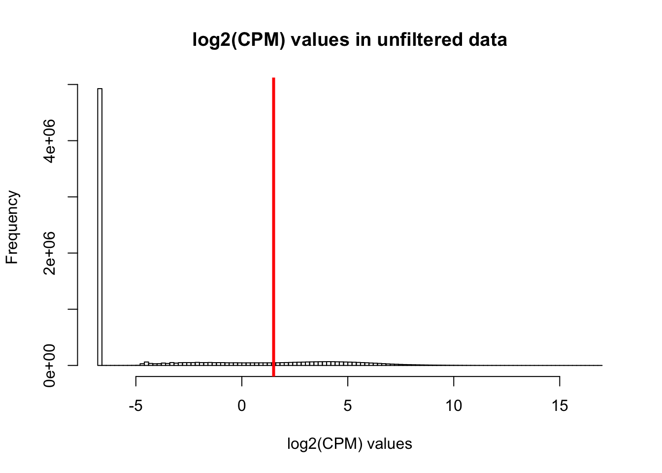

Expand here to see past versions of unnamed-chunk-2-1.png:

Version	Author	Date
7bcd123	Lauren Blake	2018-11-15

hist(cpm, main = "log2(CPM) values in unfiltered data", breaks = 100, xlab = "log2(CPM) values", ylim = c(0, 100000))
abline(v = expr_cutoff, col = "red", lwd = 3)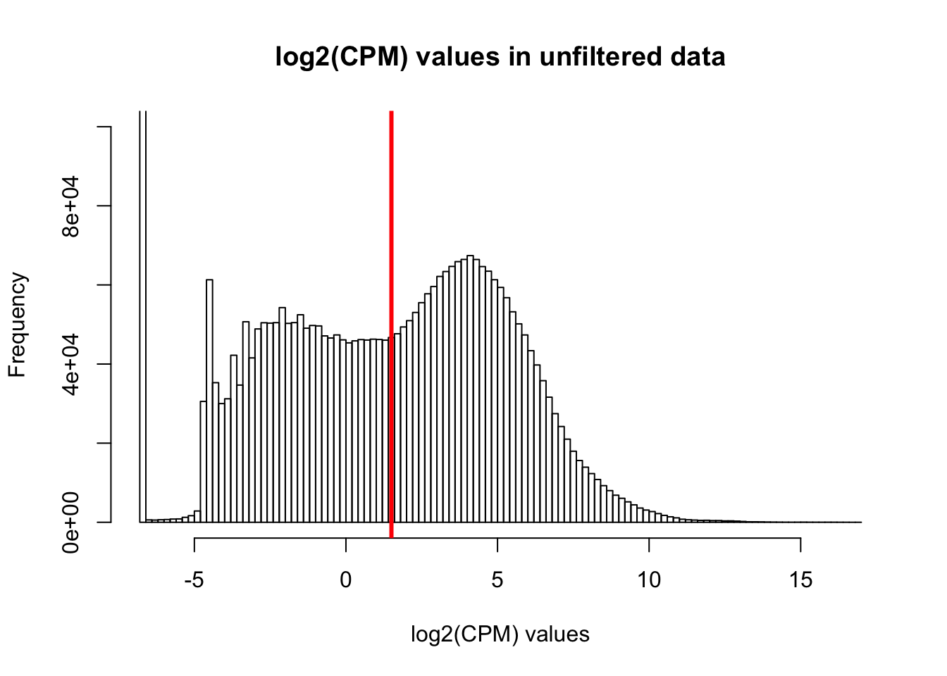

Expand here to see past versions of unnamed-chunk-2-2.png:

Version	Author	Date
7bcd123	Lauren Blake	2018-11-15

# Basic filtering
cpm_filtered <- (rowSums(cpm > 1.5) > 72)

genes_in_cutoff <- cpm[cpm_filtered==TRUE,]

hist(as.numeric(unlist(genes_in_cutoff)), main = "log2(CPM) values in filtered data", breaks = 100, xlab = "log2(CPM) values")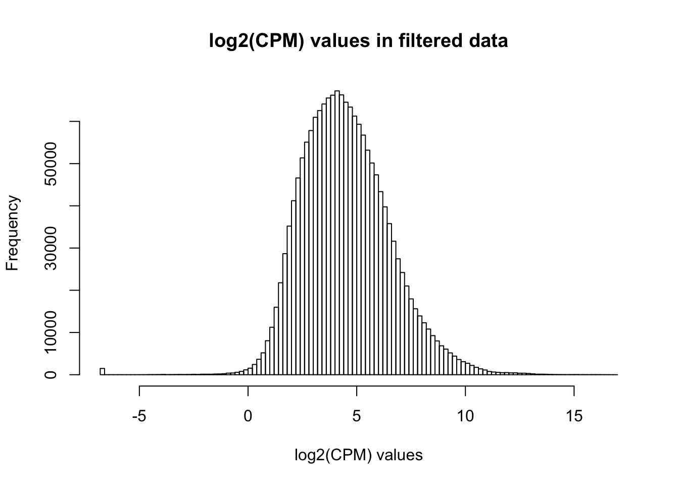

Expand here to see past versions of unnamed-chunk-2-3.png:

Version	Author	Date
7bcd123	Lauren Blake	2018-11-15

# Find the original counts of all of the genes that fit the criteria 

counts_genes_in_cutoff <- salmon_counts[cpm_filtered==TRUE,]
dim(counts_genes_in_cutoff)

[1] 11501   144

# Filter out hemoglobin

counts_genes_in_cutoff <-  counts_genes_in_cutoff[which( rownames(counts_genes_in_cutoff) != "HBB" ),]
counts_genes_in_cutoff <-  counts_genes_in_cutoff[which( rownames(counts_genes_in_cutoff) != "HBA2" ),]
counts_genes_in_cutoff <-  counts_genes_in_cutoff[which( rownames(counts_genes_in_cutoff) != "HBA1" ),]

# Take the TMM of the counts only for the genes that remain after filtering

dge_in_cutoff <- DGEList(counts=as.matrix(counts_genes_in_cutoff), genes=rownames(counts_genes_in_cutoff), group = as.character(t(clinical_sample$Individual)))
dge_in_cutoff <- calcNormFactors(dge_in_cutoff)

cpm_in_cutoff <- cpm(dge_in_cutoff, normalized.lib.sizes=TRUE, log=TRUE)

pca_genes <- prcomp(t(cpm_in_cutoff), scale = T, retx = TRUE, center = TRUE)

matrixpca <- pca_genes$x
PC1 <- matrixpca[,1]
PC2 <- matrixpca[,2]
pc3 <- matrixpca[,3]
pc4 <- matrixpca[,4]
pc5 <- matrixpca[,5]

pcs <- data.frame(PC1, PC2, pc3, pc4, pc5)

summary <- summary(pca_genes)

head(summary$importance[2,1:5])

    PC1     PC2     PC3     PC4     PC5 
0.25084 0.12998 0.08768 0.05670 0.03298 

norm_count <- ggplot(data=pcs, aes(x=PC1, y=PC2, color= as.factor(clinical_sample$Time))) + geom_point(aes(colour = as.factor(clinical_sample$Time))) + ggtitle("PCA of normalized counts") + scale_color_discrete(name = "Time")

plot_grid(norm_count)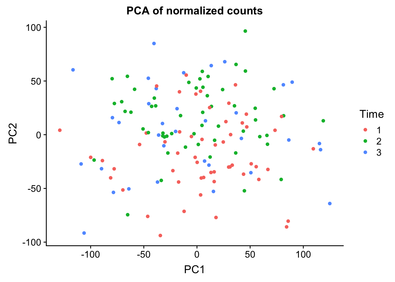

Expand here to see past versions of unnamed-chunk-2-4.png:

Version	Author	Date
7bcd123	Lauren Blake	2018-11-15

clinical_sample[,1] <- as.factor(clinical_sample[,1])

clinical_sample[,2] <- as.factor(clinical_sample[,2])

clinical_sample[,4] <- as.factor(clinical_sample[,4])

clinical_sample[,5] <- as.factor(clinical_sample[,5])

clinical_sample[,6] <- as.factor(clinical_sample[,6])


# Create the design matrix

# Use the standard treatment-contrasts parametrization. See Ch. 9 of limma
# User's Guide.

design <- model.matrix(~as.factor(Time) + Age + as.factor(Race) + as.factor(BE_GROUP) + as.factor(psychmeds) + RBC + AN + AE + AL  + RIN, data = clinical_sample)
colnames(design) <- c("Intercept", "Time2", "Time3", "Race3", "Race5", "Age", "BE", "Psychmeds", "RBC", "AN", "AE", "AL", "RIN")


# Fit model 

# Model individual as a random effect.
# Recommended to run both voom and duplicateCorrelation twice.
# https://support.bioconductor.org/p/59700/#67620

cpm.voom <- voom(dge_in_cutoff, design, normalize.method="none")
#check_rel <- duplicateCorrelation(cpm.voom, design, block = clinical_sample$Individual)
check_rel_correlation <-  0.1179835
cpm.voom.corfit <- voom(dge_in_cutoff, design, normalize.method="none", plot = TRUE, block = clinical_sample$Individual, correlation = check_rel_correlation)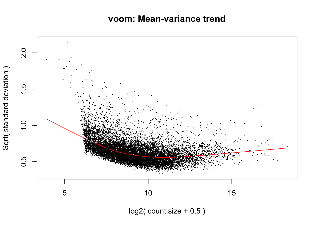

Expand here to see past versions of unnamed-chunk-2-5.png:

Version	Author	Date
7bcd123	Lauren Blake	2018-11-15

#check_rel <- duplicateCorrelation(cpm.voom.corfit, design, block = clinical_sample$Individual)
check_rel_correlation <- 0.1188083

plotDensities(cpm.voom.corfit[,1])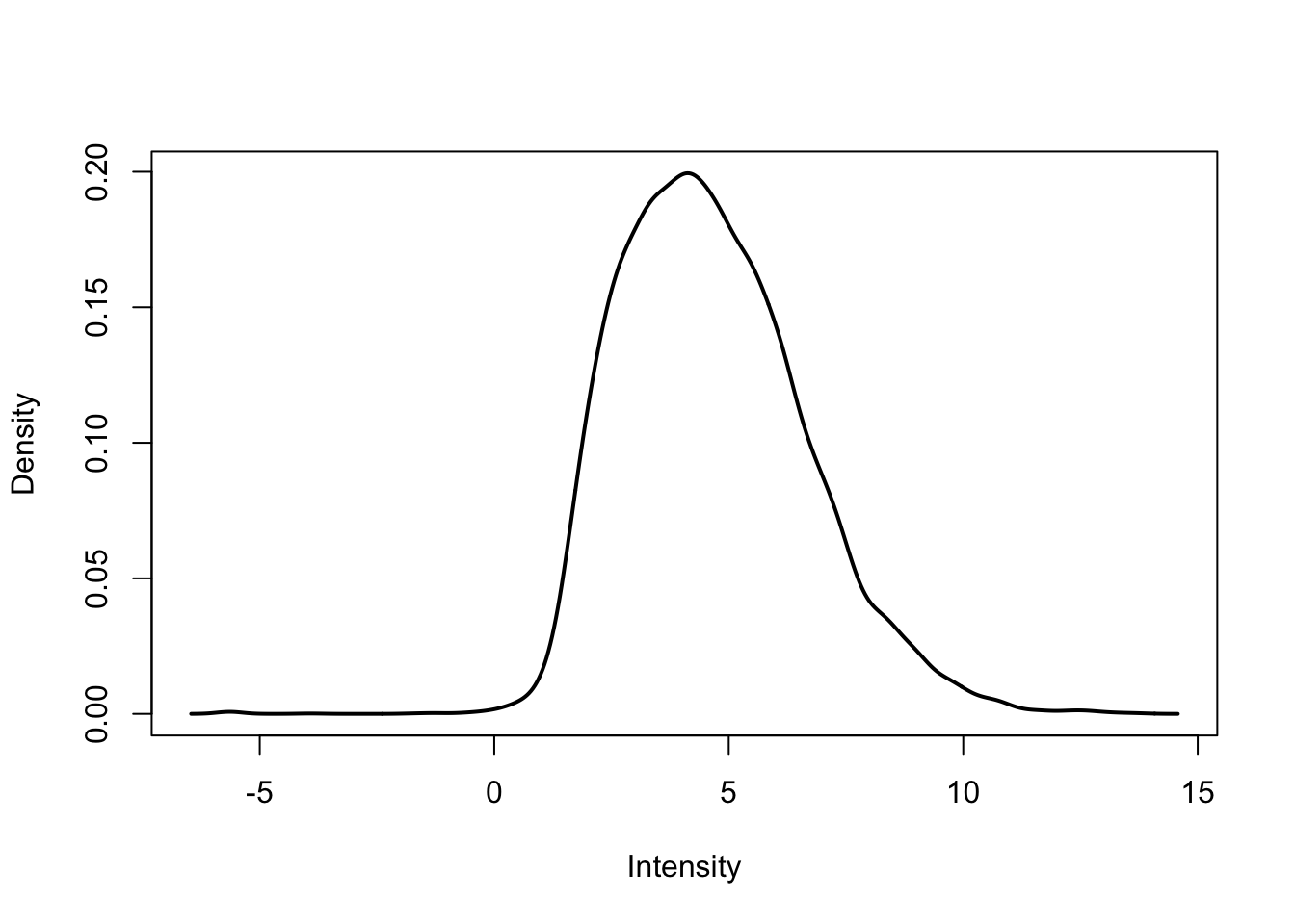

Expand here to see past versions of unnamed-chunk-2-6.png:

Version	Author	Date
7bcd123	Lauren Blake	2018-11-15

plotDensities(cpm.voom.corfit[,2])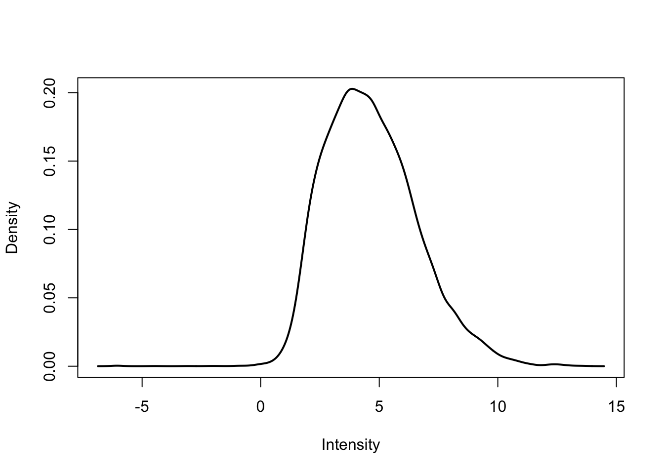

Expand here to see past versions of unnamed-chunk-2-7.png:

Version	Author	Date
7bcd123	Lauren Blake	2018-11-15

plotDensities(cpm.voom.corfit[,3])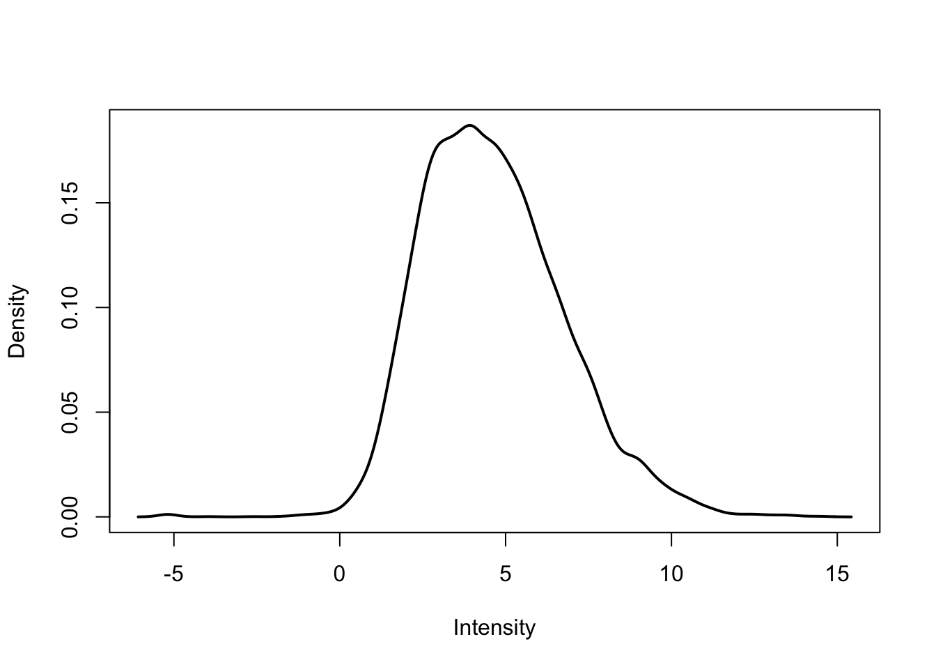

Expand here to see past versions of unnamed-chunk-2-8.png:

Version	Author	Date
7bcd123	Lauren Blake	2018-11-15

pca_genes <- prcomp(t(cpm.voom.corfit$E), scale = T, retx = TRUE, center = TRUE)

matrixpca <- pca_genes$x
PC1 <- matrixpca[,1]
PC2 <- matrixpca[,2]
pc3 <- matrixpca[,3]
pc4 <- matrixpca[,4]
pc5 <- matrixpca[,5]

pcs <- data.frame(PC1, PC2, pc3, pc4, pc5)

summary <- summary(pca_genes)

head(summary$importance[2,1:5])

    PC1     PC2     PC3     PC4     PC5 
0.25138 0.13024 0.08787 0.05642 0.03303 

ggplot(data=pcs, aes(x=PC1, y=PC2, color=clinical_sample$Time)) + geom_point(aes(colour = as.factor(clinical_sample$Time))) + ggtitle("PCA of normalized counts") + scale_color_discrete(name = "Time")

Expand here to see past versions of unnamed-chunk-2-9.png:

Version	Author	Date
7bcd123	Lauren Blake	2018-11-15

# Run lmFit and eBayes in limma

fit <- lmFit(cpm.voom.corfit, design, block=clinical_sample$Individual, correlation=check_rel_correlation)

# In the contrast matrix, have the time points

cm1 <- makeContrasts(Time1v2 = Time2, Time2v3 = Time3 - Time2, levels = design)

#cm1 <- makeContrasts(Time1v2 = Time2, Time2v3 = Time3, levels = design)

# Fit the new model
diff_species <- contrasts.fit(fit, cm1)
fit1 <- eBayes(diff_species)

FDR_level <- 0.05

Time1v2 =topTable(fit1, coef=1, adjust="BH", number=Inf, sort.by="none")
Time2v3 =topTable(fit1, coef=2, adjust="BH", number=Inf, sort.by="none")

#plot(fit1$coefficients[,1], fit1$coefficients[,2])
plot(Time1v2$logFC, Time2v3$logFC)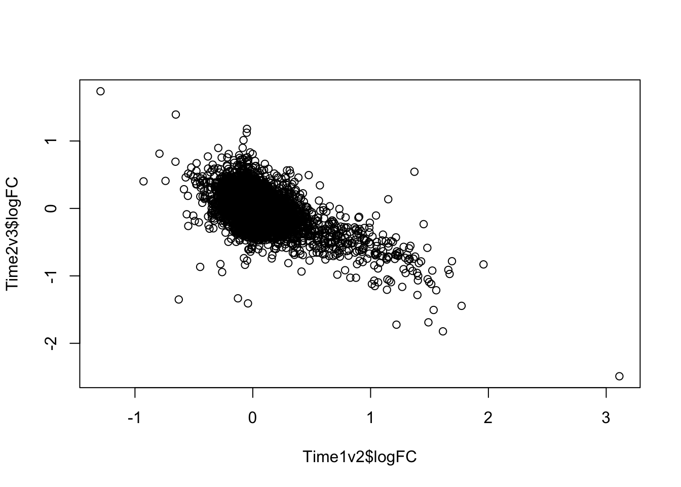

Expand here to see past versions of unnamed-chunk-2-10.png:

Version	Author	Date
7bcd123	Lauren Blake	2018-11-15

plot(Time1v2$t, Time2v3$t)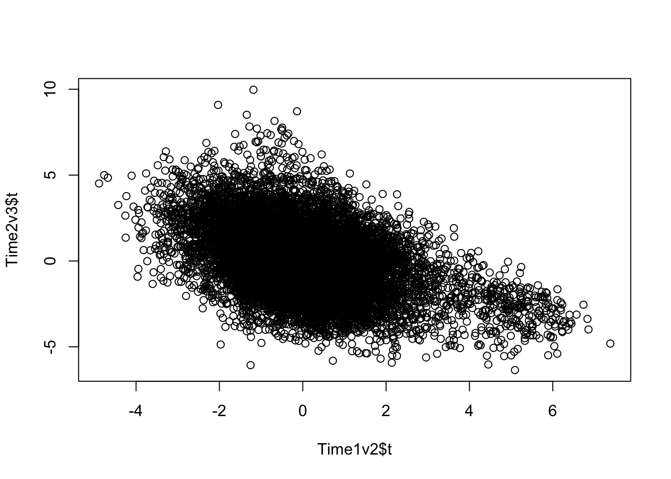

Expand here to see past versions of unnamed-chunk-2-11.png:

Version	Author	Date
7bcd123	Lauren Blake	2018-11-15

plot(Time1v2$adj.P.Val, Time2v3$adj.P.Val)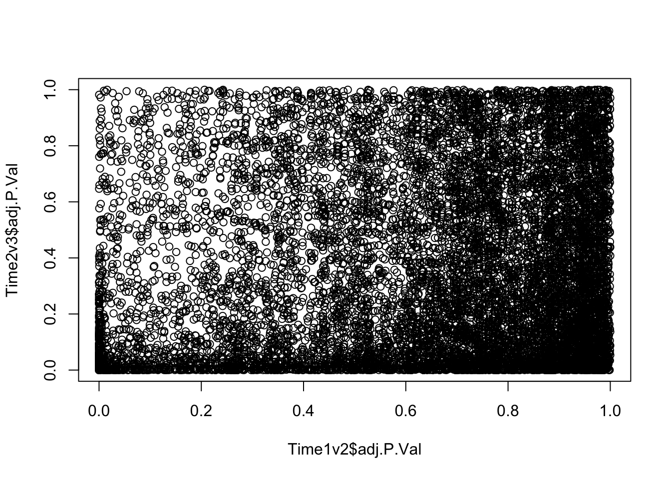

Expand here to see past versions of unnamed-chunk-2-12.png:

Version	Author	Date
7bcd123	Lauren Blake	2018-11-15

dim(Time1v2[which(Time1v2$adj.P.Val < FDR_level),])

[1] 545   7

dim(Time2v3[which(Time2v3$adj.P.Val < FDR_level),])

[1] 2272    7

head(topTable(fit1, coef=1, adjust="BH", number=100, sort.by="T"))

          genes     logFC   AveExpr        t      P.Value    adj.P.Val
DCAF6     DCAF6 0.6665640  5.416600 7.379580 1.431162e-11 1.645551e-07
RNF10     RNF10 1.0377194  8.797228 6.855830 2.272978e-10 9.869232e-07
CTNNAL1 CTNNAL1 1.4096235  1.933041 6.831796 2.575030e-10 9.869232e-07
ALAS2     ALAS2 1.9585386 10.170073 6.735151 4.244316e-10 1.220029e-06
GPR146   GPR146 1.4288917  4.655669 6.569697 9.908589e-10 2.278579e-06
VTI1B     VTI1B 0.5255125  6.179033 6.447501 1.841373e-09 3.086557e-06
               B
DCAF6   15.90792
RNF10   13.24952
CTNNAL1 12.13729
ALAS2   12.60619
GPR146  11.85371
VTI1B   11.30170

head(topTable(fit1, coef=2, adjust="BH", number=100, sort.by="T"))

                    genes     logFC  AveExpr        t      P.Value
MPHOSPH8         MPHOSPH8 0.7255845 6.149600 9.968821 6.678677e-18
DFFA                 DFFA 0.5295244 4.523835 9.085363 1.091156e-15
RTF1                 RTF1 0.5746842 5.542158 8.715696 8.936463e-15
PURA                 PURA 0.7886715 2.727101 8.512411 2.813599e-14
RP11-83A24.2 RP11-83A24.2 1.0124542 2.878809 8.153240 2.094359e-13
ZNF791             ZNF791 0.5775827 4.143783 7.827481 1.262969e-12
                adj.P.Val        B
MPHOSPH8     7.679143e-14 29.98284
DFFA         6.273054e-12 24.98292
RTF1         3.425048e-11 23.04615
PURA         8.087690e-11 21.35605
RP11-83A24.2 4.816188e-10 19.59222
ZNF791       2.420270e-09 18.21632

Make a Venn Diagram of the DE genes

# FDR 1%
FDR_level <- 0.01

Time12 <- rownames(Time1v2[which(Time1v2$adj.P.Val < FDR_level),])

Time23 <- rownames(Time2v3[which(Time2v3$adj.P.Val < FDR_level),])

mylist <- list()
mylist[["DE T1 to T2"]] <- Time12
mylist[["DE T2 to T3"]] <- Time23

# Make as pdf 
Four_comp <- venn.diagram(mylist, filename= NULL, main="DE genes between timepoints (1% FDR)", cex=1.5 , fill = NULL, lty=1, height=2000, width=2000, rotation.degree = 180, scaled = FALSE, cat.pos = c(0,0))

grid.draw(Four_comp)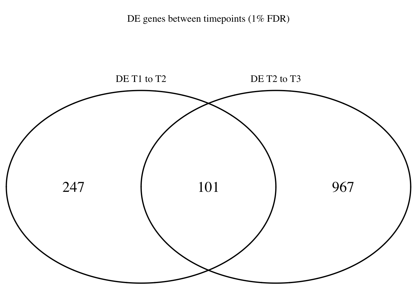

Expand here to see past versions of unnamed-chunk-3-1.png:

Version	Author	Date
7bcd123	Lauren Blake	2018-11-15

dev.off()

null device 
          1 

#pdf(file = "~/Dropbox/Figures/DET1_T2_change_weight_FDR1.pdf")
#  grid.draw(Four_comp)
#dev.off()

# FDR 5%

FDR_level <- 0.05
Time12 <- rownames(Time1v2[which(Time1v2$adj.P.Val < FDR_level),])

Time23 <- rownames(Time2v3[which(Time2v3$adj.P.Val < FDR_level),])

mylist <- list()
mylist[["DE T1 to T2"]] <- Time12
mylist[["DE T2 to T3"]] <- Time23

# Make as pdf 
Four_comp <- venn.diagram(mylist, filename= NULL, main="DE genes between timepoints (5% FDR)", cex=1.5 , fill = NULL, lty=1, height=2000, width=2000, rotation.degree = 180, scaled = FALSE, cat.pos = c(0,0))

grid.draw(Four_comp)

Expand here to see past versions of unnamed-chunk-4-1.png:

Version	Author	Date
7bcd123	Lauren Blake	2018-11-15

dev.off()

null device 
          1 

#pdf(file = "~/Dropbox/Figures/DET1_T2_change_weight_FDR5.pdf")
#  grid.draw(Four_comp)
#dev.off()

Session information

sessionInfo()

R version 3.4.3 (2017-11-30)
Platform: x86_64-apple-darwin15.6.0 (64-bit)
Running under: OS X El Capitan 10.11.6

Matrix products: default
BLAS: /Library/Frameworks/R.framework/Versions/3.4/Resources/lib/libRblas.0.dylib
LAPACK: /Library/Frameworks/R.framework/Versions/3.4/Resources/lib/libRlapack.dylib

locale:
[1] en_US.UTF-8/en_US.UTF-8/en_US.UTF-8/C/en_US.UTF-8/en_US.UTF-8

attached base packages:
[1] grid      stats     graphics  grDevices utils     datasets  methods  
[8] base     

other attached packages:
[1] cowplot_0.9.3       ggplot2_3.0.0       VennDiagram_1.6.20 
[4] futile.logger_1.4.3 edgeR_3.20.9        limma_3.34.9       

loaded via a namespace (and not attached):
 [1] Rcpp_0.12.18         bindr_0.1.1          compiler_3.4.3      
 [4] pillar_1.3.0         formatR_1.5          git2r_0.23.0        
 [7] plyr_1.8.4           workflowr_1.1.1      R.methodsS3_1.7.1   
[10] futile.options_1.0.1 R.utils_2.7.0        tools_3.4.3         
[13] digest_0.6.16        evaluate_0.11        tibble_1.4.2        
[16] gtable_0.2.0         lattice_0.20-35      pkgconfig_2.0.2     
[19] rlang_0.2.2          yaml_2.2.0           bindrcpp_0.2.2      
[22] withr_2.1.2          stringr_1.3.1        dplyr_0.7.6         
[25] knitr_1.20           tidyselect_0.2.4     locfit_1.5-9.1      
[28] rprojroot_1.3-2      glue_1.3.0           R6_2.2.2            
[31] rmarkdown_1.10       purrr_0.2.5          lambda.r_1.2.3      
[34] magrittr_1.5         whisker_0.3-2        backports_1.1.2     
[37] scales_1.0.0         htmltools_0.3.6      assertthat_0.2.0    
[40] colorspace_1.3-2     labeling_0.3         stringi_1.2.4       
[43] lazyeval_0.2.1       munsell_0.5.0        crayon_1.3.4        
[46] R.oo_1.22.0